ReLU, GELU, Swish

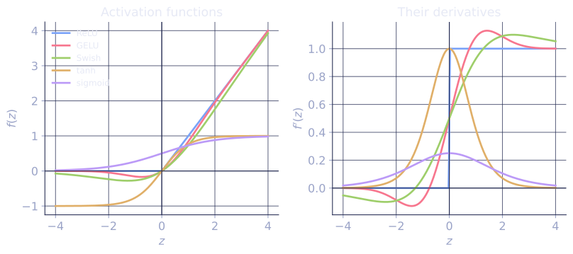
The choice of nonlinearity inside a network looks small but has outsized effects on training. ReLU dominated for a decade because of its gradient behavior; GELU and Swish are smooth variants that show small but consistent wins in Transformers. The dead-ReLU failure mode explains why the family exists at all.

ReLU

Gradient: $1$ if $z > 0$, $0$ if $z < 0$, undefined at $z = 0$ (use 0 or 1 by convention; it does not matter in practice)[1].

Why it dominated:

• Cheap. One max per element.
• Non-saturating for positive inputs. Unlike sigmoid or tanh, gradients do not vanish for large positive activations.
• Sparse activations. About half of units are zero on average, which can be a form of implicit regularization.

Dead ReLU

A ReLU unit with a negative pre-activation for every training example has zero gradient and no path to escape. The unit is dead and contributes nothing to the network from that point on.

Causes:

• Bad initialization (the next lesson fixes this).
• Learning rate too large during a noisy gradient step that drove the bias deeply negative.

Empirically, well-initialized ReLU networks have a small fraction of dead units that does not grow over training[2]. Pathological cases (e.g. extreme learning rates) can kill 50%+ of the units.

Leaky ReLU and PReLU

Leaky ReLU never zeros the gradient:

A small leak (typically 0.01) lets dead units slowly come back. PReLU treats the leak slope as a learnable parameter. Both work but rarely beat plain ReLU enough to justify the extra complexity.

ELU and SELU

ELU uses a smooth negative branch:

SELU combines ELU with a carefully chosen scale to give self-normalizing behavior: under the right initialization, layer activations stay roughly mean-zero and variance-one without explicit normalization layers. Pretty in theory; less popular in practice because modern architectures use explicit normalization (next lesson).

GELU

The activation that powers most Transformers:

where $\Phi$ is the standard normal CDF. Intuition: a stochastic gate that drops the input with probability $1 - \Phi(z)$. Smooth, monotone-ish, and approximately $z$ for large positive $z$. The exact form uses the erf function; a common tanh-based approximation is

GELU consistently outperforms ReLU in Transformer feed-forward layers, typically by 0.1-0.5 perplexity points in language modeling[3]. The reason is debated; the smooth gating around zero seems to matter.

Swish (SiLU)

with $\sigma$ the logistic sigmoid. Closely related to GELU (visually almost identical for $|z| < 3$). Discovered by neural architecture search, justified by ablations rather than theory. Modern papers refer to it as SiLU (sigmoid linear unit).

Practical recipe

• CNNs: ReLU is fine; switch to Swish/GELU if you have a tuning budget and care about the last few percentage points.
• Transformers: GELU is the default. Switching to Swish is rarely meaningful; switching to ReLU loses noticeable performance.
• Anywhere with normalization layers and residual connections: the activation choice matters less.

Check it on arrays

import numpy as np

z = np.linspace(-4, 4, 100)

def relu(z):  return np.maximum(0, z)
def gelu(z):  return 0.5 * z * (1 + np.tanh(np.sqrt(2 / np.pi) * (z + 0.044715 * z**3)))
def swish(z): return z / (1 + np.exp(-z))
def elu(z, alpha=1.0): return np.where(z >= 0, z, alpha * (np.exp(z) - 1))

# Compare derivatives at zero: this is what matters for "smooth around zero"
def num_deriv(f, z, eps=1e-5): return (f(z + eps) - f(z - eps)) / (2 * eps)
print(f"derivative at z=0:")
# ReLU is not differentiable at 0; centered finite differences average the
# left (0) and right (1) one-sided derivatives, so they print 0.5 at the kink.
print(f"  ReLU:  {num_deriv(relu, 0.0):.4f}  (centered diff averages left=0 and right=1)")
print(f"  GELU:  {num_deriv(gelu, 0.0):.4f}")
print(f"  Swish: {num_deriv(swish, 0.0):.4f}")
print(f"  ELU:   {num_deriv(elu, 0.0):.4f}")

# Demonstrate dead ReLU: with bad initialization, a fraction of units have
# all-negative pre-activations and produce zero gradient forever. X is zero-
# mean so shifting W's mean does nothing; the bias is what kills units.
rng = np.random.default_rng(0)
N, d, hidden = 500, 20, 256
X = rng.normal(size=(N, d))
W_bad = rng.normal(scale=0.5, size=(d, hidden))
b_bad = rng.normal(loc=-6.0, scale=1.0, size=hidden)        # biases pushed strongly negative
preact = X @ W_bad + b_bad
dead_units = ((preact <= 0).all(axis=0)).sum()
print(f"\ndead ReLU units (with deliberately bad init): {dead_units} / {hidden}")

ReLU is non-differentiable at zero (its left-derivative is 0 and its right-derivative is 1); the subdifferential convention picks one of these, typically 0, while a centered finite-difference averages them and prints 0.5. GELU and Swish are smooth at zero. The bad-initialization demo shows how a substantial fraction of units can land in the dead region from a single poor initialization.

Exercises

Exercise 1. Compute $\operatorname{ReLU}(z)$ and its derivative for $z \in \{-2,\ -0.5,\ 0,\ 1.5\}$, using the convention that the derivative at $z = 0$ is $0$.

Exercise 2. Leaky ReLU with slope $0.01$ never zeros its gradient, so it has no dead-unit region. Show this: for what pre-activations $z$ is the derivative of $\operatorname{LeakyReLU}(z) = \max(0.01 z, z)$ equal to zero?

Exercise 3 (code). The Swish derivative is $\sigma(z) + z\,\sigma(z)(1 - \sigma(z))$ where $\sigma$ is the logistic sigmoid. Verify this analytic form against a central finite difference of $\operatorname{Swish}(z) = z\,\sigma(z)$ across a range of $z$.

import numpy as np

def sigmoid(z): return 1.0 / (1.0 + np.exp(-z))
def swish(z):   return z * sigmoid(z)
def swish_grad(z):
    s = sigmoid(z)
    return s + z * s * (1 - s)

z = np.linspace(-5, 5, 200)
analytic = swish_grad(z)

eps = 1e-6
fd = (swish(z + eps) - swish(z - eps)) / (2 * eps)

assert np.max(np.abs(analytic - fd)) < 1e-7
print("max |analytic - finite diff|:", np.max(np.abs(analytic - fd)))

The next lesson fixes this systematically with Xavier and He initialization.

References

- [1]Nair, V., & Hinton, G. E. (2010). "Rectified linear units improve restricted Boltzmann machines". ICML. The introduction of ReLU as a hidden-unit nonlinearity.↩
- [2]He, K., Zhang, X., Ren, S., & Sun, J. (2015). "Delving deep into rectifiers: surpassing human-level performance on ImageNet classification". ICCV. arXiv:1502.01852. Analyzes ReLU-family units (including the dead-unit regime) and the initialization that matches them.↩
- [3]Goodfellow, I., Bengio, Y., & Courville, A. (2016). Deep Learning, §6.3 (Hidden Units). MIT Press. Survey of activation choices and their gradient behavior.↩