BatchNorm, LayerNorm, RMSNorm

Normalization layers actively rescale activations to a target mean and variance, then learn a per-channel affine. The result: training is stable across initializations, learning rates can be larger, and very deep networks become feasible. The three dominant variants (BatchNorm, LayerNorm, RMSNorm) differ in which axes they normalize over, and that choice is dictated by the network's batch and sequence structure.

BatchNorm

For each feature channel, normalize across the batch dimension:

Then a learned affine $y_{i,c} = \gamma_c\, \hat x_{i,c} + \beta_c$ restores any scale and shift the next layer wants. The statistics are computed per batch during training; running averages are kept for inference[1].

Strengths: enabled the original ResNet, lets you use larger learning rates, smooths the loss landscape. Most CNN architectures rely on it.

Failure modes:

• Small batches (e.g. 1 or 2): per-batch statistics are noisy and training degrades. GroupNorm (a variant) helps here.
• Train/eval mismatch: the running statistics seen at inference differ from per-batch statistics seen at training, so eval-mode is different from train-mode in subtle ways.
• Variable-length sequences: batch-dimension stats blend padding tokens with real ones. Not used in Transformers.

LayerNorm

For each example, normalize across the feature dimension:

The statistics are computed per-example, so they do not depend on the batch. Eval-mode = train-mode, and batch size 1 works fine[2].

Strengths: works on variable-length sequences, no train/eval mismatch, naturally handles small batches.

Where: Transformers (everywhere; pre-LN is standard), RNNs, attention-based architectures. Most modern non-CNN models use LayerNorm.

RMSNorm

LayerNorm normalizes by the standard deviation (subtract mean, divide by sd). RMSNorm drops the mean centering and uses only the root mean square:

Cheaper (no mean subtraction, no centered variance) and empirically as good as LayerNorm on language tasks. The default in modern LLM architectures (LLaMA, Mistral, most recent recipes).

Group, Instance, and other variants

• GroupNorm: split channels into $G$ groups and normalize within each group across the spatial dims. Bridges BatchNorm and LayerNorm for vision; useful when batch is small.
• InstanceNorm: normalize per-example, per-channel across spatial dims. Used in style transfer.
• Weight Normalization / Weight Standardization: normalize the weights rather than activations. Less popular but still around.

The choice is largely architectural: BatchNorm for vision CNNs at decent batch sizes; LayerNorm or RMSNorm for Transformers and sequence models[3].

Pre-norm vs post-norm

In residual networks, where to place the normalization matters:

• Post-norm (original Transformer): x = LN(x + sublayer(x)). The norm sits after the residual addition.
• Pre-norm (now standard): x = x + sublayer(LN(x)). The norm sits before the sublayer.

Pre-norm is dramatically more stable in very deep networks, because the residual path stays unnormalized (gradients flow cleanly) and the sublayer input is normalized. Almost all modern Transformers use pre-norm.

What it gives you

Empirically:

• 2-10x faster convergence.
• Robust to learning rates spanning 1-2 orders of magnitude.
• Enables 100+ layer networks (without norm, gradient flow breaks down).

The catch: a normalization layer adds compute and parameter count (typically negligible relative to the linear layers it sits between) and some non-locality (the normalization couples examples in a batch for BN).

Check it on arrays

import numpy as np

rng = np.random.default_rng(0)

def batch_norm(X, eps=1e-5):
    """Across batch, per channel. Returns (out, mean, var)."""
    mu = X.mean(axis=0); var = X.var(axis=0)
    return (X - mu) / np.sqrt(var + eps), mu, var

def layer_norm(X, eps=1e-5):
    """Per example, across feature dim."""
    mu = X.mean(axis=1, keepdims=True); var = X.var(axis=1, keepdims=True)
    return (X - mu) / np.sqrt(var + eps)

def rms_norm(X, eps=1e-5):
    """Per example, RMS only (no mean subtraction)."""
    return X / np.sqrt((X**2).mean(axis=1, keepdims=True) + eps)

N, C = 64, 16
X = rng.normal(loc=2.0, scale=3.0, size=(N, C))

bn, _, _ = batch_norm(X)
ln = layer_norm(X)
rn = rms_norm(X)

print(f"input         mean={X.mean():+.3f}, std={X.std():.3f}")
print(f"BatchNorm out mean={bn.mean():+.3f}, std={bn.std():.3f}, per-channel std std={bn.std(axis=0).std():.4f}")
print(f"LayerNorm out mean={ln.mean():+.3f}, std={ln.std():.3f}, per-example std std={ln.std(axis=1).std():.4f}")
print(f"RMSNorm   out mean={rn.mean():+.3f}, std={rn.std():.3f}, per-example RMS std={np.sqrt((rn**2).mean(axis=1)).std():.4f}")

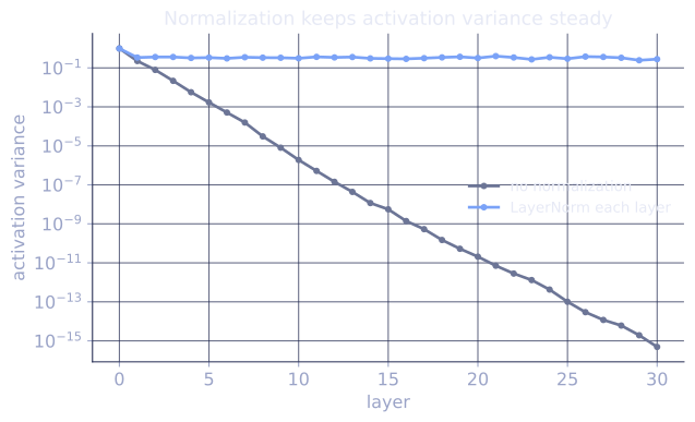
# Effect on a deep ReLU stack: with normalization the activation scale
# is preserved across many layers regardless of initialization.
def naive_init(in_dim, out_dim, rng): return rng.normal(scale=0.1, size=(in_dim, out_dim))

def deep_with_norm(use_norm, depth=30, width=64):
    h = rng.normal(size=(64, width))
    var_history = [h.var()]
    for _ in range(depth):
        W = naive_init(width, width, rng)
        z = h @ W
        if use_norm: z = layer_norm(z)
        h = np.maximum(0, z)
        var_history.append(h.var())
    return var_history

no_norm = deep_with_norm(use_norm=False)
with_norm = deep_with_norm(use_norm=True)
print(f"\nactivation variance after 30 layers (bad init):")
print(f"  no normalization: layer 5 = {no_norm[5]:.2e}, layer 30 = {no_norm[30]:.2e}")
print(f"  with LayerNorm:   layer 5 = {with_norm[5]:.3f}, layer 30 = {with_norm[30]:.3f}")

LayerNorm rescues a deep ReLU stack with deliberately bad initialization that otherwise collapses to zero.

Exercises

Exercise 1. Take the feature vector $x = (1, 2, 3, 4)$ for one example. Compute its LayerNorm output (no learned affine, $\varepsilon = 0$) and its RMSNorm output by hand, and explain why the two differ.

Exercise 2. Prove that LayerNorm is invariant to a global shift and scale of the input: for any scalars $a > 0$ and $c$, the LayerNorm of $a\,x + c$ (the same $a, c$ added to every coordinate) equals the LayerNorm of $x$, ignoring the learned affine.

Exercise 3 (code). Verify the scale-and-shift invariance from Exercise 2 numerically, and confirm that BatchNorm is not invariant to a per-example shift (because it normalizes across the batch, not the feature axis).

import numpy as np

rng = np.random.default_rng(0)

def layer_norm(X, eps=1e-5):
    mu = X.mean(axis=1, keepdims=True); var = X.var(axis=1, keepdims=True)
    return (X - mu) / np.sqrt(var + eps)

def batch_norm(X, eps=1e-5):
    mu = X.mean(axis=0); var = X.var(axis=0)
    return (X - mu) / np.sqrt(var + eps)

N, C = 8, 6
X = rng.normal(size=(N, C))

# Global affine transform of each example: a * x + c
a, c = 3.0, 5.0
X_aff = a * X + c

# LayerNorm is invariant (up to floating point) to per-example affine
assert np.allclose(layer_norm(X), layer_norm(X_aff), atol=1e-4)

# BatchNorm shifting one example's features changes that example's output,
# because the per-channel batch mean moves.
X_shift = X.copy()
X_shift[0] += 10.0
assert not np.allclose(batch_norm(X)[0], batch_norm(X_shift)[0])

print("LayerNorm invariant to per-example affine:",
      np.allclose(layer_norm(X), layer_norm(X_aff), atol=1e-4))
print("BatchNorm changed for shifted example:",
      not np.allclose(batch_norm(X)[0], batch_norm(X_shift)[0]))

The next lesson covers two other training-stability tools: dropout and weight decay.

References

- [1]Ioffe, S., & Szegedy, C. (2015). "Batch normalization: accelerating deep network training by reducing internal covariate shift". ICML. arXiv:1502.03167. Introduces BatchNorm with per-batch statistics and inference-time running averages.↩
- [2]Ba, J. L., Kiros, J. R., & Hinton, G. E. (2016). "Layer normalization". arXiv:1607.06450. Normalizes per-example across features, removing the batch dependence.↩
- [3]Goodfellow, I., Bengio, Y., & Courville, A. (2016). Deep Learning, §8.7.1 (Batch Normalization). MIT Press. Normalization as an optimization aid in deep networks.↩