Xavier and He initialization

A randomly-initialized network's forward pass is a sequence of linear maps; its output variance grows or shrinks geometrically with depth unless each layer's variance is carefully matched to the activation that follows. Xavier (Glorot) for tanh and He for ReLU give the variance-preserving formulas. Bad initialization stalls training before gradient descent has a chance.

The variance-propagation problem

Treat the inputs to layer $\ell$ as zero-mean random variables with variance $\operatorname{Var}(h^{(\ell-1)}_j) = v_{\ell-1}$. After the linear map $z^{(\ell)} = W^{(\ell)} h^{(\ell-1)}$, assuming independent zero-mean weights with variance $\sigma_W^2$:

where $d_{\ell-1}$ is the input dimension. If we want $\operatorname{Var}(z^{(\ell)}_i) = v_{\ell-1}$, the weight variance must be

For the activation that follows, the variance contracts or expands by a factor that depends on the nonlinearity, which is where Xavier and He differ.

Xavier (Glorot) for tanh and sigmoid

For tanh, around zero $\tanh(z) \approx z$, so the activation approximately preserves variance for small inputs. The Glorot initialization compromises between forward variance preservation (needs $\sigma_W^2 = 1/d_{\ell-1}$) and backward variance preservation (needs $\sigma_W^2 = 1/d_\ell$) by averaging[1]:

In code: $W_{ij} \sim \mathcal{N}(0, \sigma_W^2)$ or $W_{ij} \sim \text{Uniform}(-\sqrt{6/(d_{\ell-1} + d_\ell)},\ \sqrt{6/(d_{\ell-1} + d_\ell)})$.

He for ReLU

ReLU zeros out the negative half of its inputs. For a zero-mean Gaussian $z$, $\mathbb{E}[\operatorname{ReLU}(z)^2] = \mathbb{E}[z^2]/2 = \operatorname{Var}(z)/2$. So ReLU halves the variance. To compensate, the weight variance must double:

In code: $W_{ij} \sim \mathcal{N}(0, 2/d_{\ell-1})$[2]. He initialization is the standard for any ReLU-family network (including GELU and Swish, which behave similarly enough that He's factor of 2 is a fine default).

Why bad initialization stalls

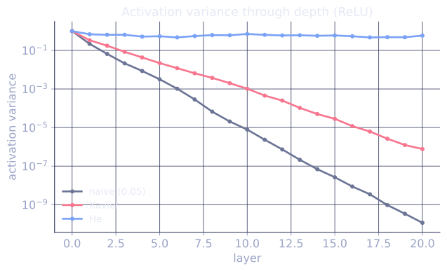
If $\sigma_W^2$ is too small, $\operatorname{Var}(z^{(\ell)})$ shrinks geometrically: by layer 10, activations are vanishingly small, and the backward pass propagates zero gradients. The network is a constant function in practice; no learning happens.

If $\sigma_W^2$ is too large, $\operatorname{Var}(z^{(\ell)})$ grows geometrically: by layer 10, activations saturate the nonlinearity (for tanh) or land in extreme regions (for ReLU). Backward gradients are unstable. Loss is NaN within a few steps.

The right initialization keeps the variance roughly constant across layers, so a 30-layer network has the same activation scale at layer 30 as at layer 1.

What changed with normalization

Once BatchNorm or LayerNorm is inserted between layers, the initialization matters much less: normalization layers actively rescale activations to mean-zero, variance-one regardless of what came before. Modern networks rely on this safety net, so they can be slightly more forgiving with initialization than pre-normalization architectures.

But the principle still applies: without normalization, careful initialization is the difference between a network that trains and one that does not.

Initialization for biases and special layers

• Biases: initialize to zero, almost always.
• Output layer for classification: same rule as hidden layers; the softmax will sort itself out.
• Output layer for regression: zero-init the weights so initial predictions are zero; the loss then comes purely from the target.
• LSTM/GRU forget gates: initialize bias to a positive value ($+1$ or $+2$) so the gates start mostly open and gradients propagate.
• Transformer attention output projection: zero-init or small init helps stability in early training (used in many recent recipes).

Check it on arrays

import numpy as np

rng = np.random.default_rng(0)

def run_network(init_fn, depth=20, width=256, n_samples=1024, activation="relu"):
    """Propagate random unit-variance inputs through `depth` layers with
    the given initialization, and report the per-layer activation variance."""
    X = rng.normal(size=(n_samples, width))
    var = [X.var()]
    h = X
    for _ in range(depth):
        W = init_fn(width, width, rng)
        z = h @ W
        if activation == "relu":
            h = np.maximum(0, z)
        elif activation == "tanh":
            h = np.tanh(z)
        var.append(h.var())
    return var

def naive(in_dim, out_dim, rng): return rng.normal(scale=0.05, size=(in_dim, out_dim))
def xavier(in_dim, out_dim, rng):
    return rng.normal(scale=np.sqrt(2 / (in_dim + out_dim)), size=(in_dim, out_dim))
def he(in_dim, out_dim, rng):
    return rng.normal(scale=np.sqrt(2 / in_dim), size=(in_dim, out_dim))

# ReLU network: He should keep variance stable, others should shrink/grow
print("Per-layer activation variance (depth=20, ReLU):")
for name, fn in [("naive 0.05", naive), ("Xavier", xavier), ("He", he)]:
    v = run_network(fn, activation="relu")
    print(f"  {name:>10}: layer 0={v[0]:.3f}, layer 5={v[5]:.3f}, "
          f"layer 10={v[10]:.3f}, layer 20={v[20]:.3f}")

print("\nPer-layer activation variance (depth=20, tanh):")
for name, fn in [("naive 0.05", naive), ("Xavier", xavier), ("He", he)]:
    v = run_network(fn, activation="tanh")
    print(f"  {name:>10}: layer 0={v[0]:.3f}, layer 5={v[5]:.3f}, "
          f"layer 10={v[10]:.3f}, layer 20={v[20]:.3f}")

He keeps variance stable across the depth of a ReLU network; Xavier matches it for tanh. Naive small-scale initialization collapses variance to zero within a few layers.

Exercises

Exercise 1. A linear layer has fan-in $d_{\ell-1} = 100$ and fan-out $d_\ell = 300$. Give the weight standard deviation $\sigma_W$ for He initialization and for Xavier (Glorot) initialization.

Exercise 2. Derive the ReLU variance-halving fact used by He. For a zero-mean Gaussian $z$, show that $\mathbb{E}[\operatorname{ReLU}(z)^2] = \tfrac12 \operatorname{Var}(z)$, then conclude why the weight variance must double.

Exercise 3 (code). Empirically confirm the variance-halving: pass a zero-mean unit-variance Gaussian through ReLU and check the output second moment is $\approx 0.5$. Then build a 30-layer linear-ReLU stack and assert that He init keeps the final activation variance within an order of magnitude of the input, while a naive small-scale init collapses it by many orders.

import numpy as np

# Variance-halving: E[ReLU(z)^2] = 0.5 for standard normal z
rng = np.random.default_rng(0)
z = rng.normal(size=2_000_000)
assert np.isclose((np.maximum(0, z) ** 2).mean(), 0.5, atol=1e-3)

def final_var_ratio(scale_fn, seed, depth=30, width=256, n=8192):
    rng = np.random.default_rng(seed)
    h = rng.normal(size=(n, width)); v0 = h.var()
    for _ in range(depth):
        W = rng.normal(scale=scale_fn(width), size=(width, width))
        h = np.maximum(0, h @ W)
    return h.var() / v0

he    = final_var_ratio(lambda w: np.sqrt(2 / w), seed=0)
naive = final_var_ratio(lambda w: 0.05,           seed=0)

# He holds the same order of magnitude; naive collapses toward zero
assert 0.1 < he < 10
assert naive < 1e-10
assert he / naive > 1e10
print(f"He ratio={he:.3f}, naive ratio={naive:.2e}")

The next lesson installs normalization layers that make the network self-stabilizing even when initialization is imperfect.

References

- [1]Glorot, X., & Bengio, Y. (2010). "Understanding the difficulty of training deep feedforward neural networks". AISTATS. Derives the variance-preserving (Xavier) initialization for tanh and sigmoid networks.↩
- [2]He, K., Zhang, X., Ren, S., & Sun, J. (2015). "Delving deep into rectifiers: surpassing human-level performance on ImageNet classification". ICCV. arXiv:1502.01852. Corrects the variance factor to for ReLU networks.↩