Universal approximation

A natural question: how expressive is the MLP function class? The answer is the universal approximation theorem: a single hidden layer with enough units can approximate any continuous function on a compact set, to any accuracy. The theorem says expressiveness is not a bottleneck; depth, width, and optimization are.

The statement

Theorem (Cybenko 1989, Hornik 1991). Let $\sigma: \mathbb{R} \to \mathbb{R}$ be a nonconstant, bounded, monotone-increasing continuous function (or, in modern variants, any nonpolynomial continuous function, including ReLU). For any continuous $f: K \to \mathbb{R}$ on a compact $K \subset \mathbb{R}^n$ and any $\varepsilon > 0$, there exist integers $M$, weights $w_i \in \mathbb{R}^n$, biases $b_i \in \mathbb{R}$, and output coefficients $c_i \in \mathbb{R}$ such that

A single hidden layer (width $M$, possibly very large) approximates any continuous function on a compact set[1, 2]. ReLU MLPs satisfy a corresponding theorem (Leshno et al. 1993): the only nonlinearities for which universal approximation fails are polynomials.

Why this matters less than it sounds

The theorem says expressiveness is not the bottleneck. It does not say:

• That training will find the right weights. Optimization is a separate problem (the next lessons).
• How big $M$ needs to be. For some functions, $M$ grows exponentially with input dimension or accuracy.
• That a single hidden layer is the right architecture. Depth lets the same total parameter budget represent some functions exponentially more efficiently than width can.

So in practice, the choice between a wide shallow network and a deep narrow one matters enormously, even though both are universal.

Why a sketch makes the result believable

A working intuition for one-dimensional inputs: with sigmoid-like $\sigma$ and a pair of units $(w_1, b_1), (w_2, b_2)$, you can build a bump function with controllable width and height. Stacking many bumps along the input axis approximates any continuous function by piecewise-constant blocks that look like its integral.

For multi-dimensional inputs, the construction generalizes: each unit's $w_i^\top x + b_i$ defines a hyperplane, and combinations of opposite-sign units carve out half-space differences that approximate cells.

The argument is not constructive in any useful sense at high dimension, but it makes "infinite hidden units can fit any function" believable from first principles.

Depth vs width

Modern deep learning is empirically about depth, not width. Two results explain why:

• Constructive depth advantage. For functions like compositions of many simple primitives (parity, multi-step decisions), a shallow network needs exponentially many units while a deep one needs polynomially many.
• Optimization friendliness. Deep networks with residual connections train more easily than equivalently-sized wide shallow networks, even when both have the same parameter count.

Neither is a corollary of the universal approximation theorem. The theorem says "deep is not necessary in principle"; experiments show "deep is hugely useful in practice".

Beyond MLPs

Universal approximation theorems exist for:

• CNNs (with enough channels and depth).
• Transformers (with enough heads and depth).
• GNNs (with caveats about distinguishing isomorphic graphs: Weisfeiler-Leman tests).

In every case, the theorem is comforting but does not predict practical performance. Architecture matters because of inductive bias, optimization, and sample efficiency, not because the universal-approximation class is too small.

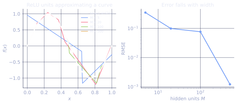
Check it on arrays

A pictorial check: build a wide one-hidden-layer ReLU network with random weights, fit only the output coefficients, and watch it approximate a nontrivial target.

import numpy as np

rng = np.random.default_rng(0)

# Target: sin(2 pi x)
x_train = np.linspace(0, 1, 200)
y_train = np.sin(2 * np.pi * x_train)

def features(x, M, rng):
    # Random hidden layer: x -> ReLU(w * x + b)
    w = rng.normal(scale=5.0, size=M)
    b = rng.uniform(-2, 2, size=M)
    return np.maximum(0.0, np.outer(x, w) + b)

for M in [5, 20, 100, 500]:
    Phi = features(x_train, M, rng)
    # Fit output coefficients by least squares
    c, *_ = np.linalg.lstsq(Phi, y_train, rcond=None)
    y_hat = Phi @ c
    rmse = np.sqrt(np.mean((y_hat - y_train)**2))
    print(f"M = {M:>4}: RMSE = {rmse:.4f}")

The fit improves monotonically as the hidden width grows; with enough units, a single hidden layer reproduces the sinusoid to machine-precision RMSE.

Exercises

Exercise 1. The sketch builds a bump from two sigmoidal units. For a sharp sigmoid (large slope), the combination $c\,[\sigma(s(x - a)) - \sigma(s(x - b))]$ with $a < b$ approximates a rectangular bump. State its approximate height and the interval over which it is nonzero, and explain what the height $c$ and the gap $b - a$ control.

Exercise 2. A ReLU unit is $\operatorname{ReLU}(wx + b) = \max(0, wx + b)$, a hinge. Show that a difference of two ReLU hinges produces a single "kink-up then kink-down" shape, and that with a third term you can build a triangular bump on the real line. Give the coefficients for a unit-height triangle peaking at $x = 0$ with support $[-1, 1]$.

Exercise 3 (code). Build the triangular bump from Exercise 2 with a hand-set ReLU network (no training), then verify it matches the target triangle and confirm the staircase idea: fit a small bump target $f(x) = \max(0, 1 - |x|)$ with a wider random ReLU layer and watch the error fall as width grows.

import numpy as np

rng = np.random.default_rng(0)

def relu(z): return np.maximum(0.0, z)

x = np.linspace(-2, 2, 401)
target = np.maximum(0.0, 1 - np.abs(x))    # unit triangle on [-1, 1]

# Hand-built ReLU triangle: ReLU(x+1) - 2 ReLU(x) + ReLU(x-1)
hand = relu(x + 1) - 2 * relu(x) + relu(x - 1)
assert np.allclose(hand, target, atol=1e-12)

# Staircase / random-feature fit: wider random hidden layer drives error down
def fit_rmse(M):
    w = rng.normal(scale=4.0, size=M)
    b = rng.uniform(-2, 2, size=M)
    Phi = relu(np.outer(x, w) + b)
    c, *_ = np.linalg.lstsq(Phi, target, rcond=None)
    return np.sqrt(np.mean((Phi @ c - target) ** 2))

rmses = [fit_rmse(M) for M in [4, 16, 64, 256]]
assert rmses[-1] < rmses[0]                 # error falls as width grows
print("hand-built triangle matches target exactly")
for M, r in zip([4, 16, 64, 256], rmses):
    print(f"M = {M:>3}: RMSE = {r:.4f}")

The next lesson picks the right $\sigma$ for the inner nonlinearity: ReLU and its modern variants.

References

- [1]Cybenko, G. (1989). "Approximation by superpositions of a sigmoidal function". Mathematics of Control, Signals and Systems, 2, 303-314. doi:10.1007/BF02551274. Proves universal approximation for sigmoidal single-hidden-layer networks.↩
- [2]Hornik, K., Stinchcombe, M., & White, H. (1989). "Multilayer feedforward networks are universal approximators". Neural Networks, 2(5), 359-366. doi:10.1016/0893-6080(89)90020-8. Establishes the same result for a broad class of nonlinearities.↩