Singular value decomposition

The eigendecomposition applies only to square matrices and only when a full eigenbasis exists. The singular value decomposition extends the same geometry to any matrix, square or rectangular, and always exists[1, 2]. It is the factorization that underlies PCA, low-rank approximation, pseudo-inverses, and numerical rank computation.

Constructing the SVD

Let $A \in \mathbb{R}^{m \times n}$. The matrix $A^\top A \in \mathbb{R}^{n \times n}$ is symmetric and PSD (previous lesson: $x^\top A^\top A x = \lVert Ax\rVert^2 \ge 0$). By the spectral theorem, it has a real orthonormal eigenbasis.

Step 1: diagonalize $A^\top A$.

The eigenvalues are nonnegative by PSD. Order them $\lambda_1 \ge \lambda_2 \ge \cdots \ge \lambda_n \ge 0$. The singular values are $\sigma_i = \sqrt{\lambda_i}$.

Step 2: construct the left singular vectors. For each $\sigma_i > 0$, define

These are unit vectors in $\mathbb{R}^m$: $\lVert u_i\rVert^2 = \frac{1}{\sigma_i^2} \lVert Av_i\rVert^2 = \frac{1}{\sigma_i^2} v_i^\top A^\top A v_i = \frac{\lambda_i}{\sigma_i^2} = 1$.

They are mutually orthogonal: for $i \neq j$, $\langle u_i, u_j\rangle = \frac{1}{\sigma_i\sigma_j} v_i^\top A^\top A v_j = \frac{\lambda_j}{\sigma_i\sigma_j}\langle v_i, v_j\rangle = 0$.

Extend $\{u_1, \dots, u_r\}$ (where $r$ is the rank) to an orthonormal basis $\{u_1, \dots, u_m\}$ of $\mathbb{R}^m$ by adding arbitrary orthonormal vectors.

Step 3: write $A = U\Sigma V^\top$. By construction $Av_i = \sigma_i u_i$ for $i \le r$ and $Av_i = 0$ for $i > r$ (those $v_i$ lie in $\ker A$). Collecting into matrices:

i.e. $AV = U\Sigma$, hence $A = U\Sigma V^\top$.

Here $U \in \mathbb{R}^{m \times m}$ and $V \in \mathbb{R}^{n \times n}$ are orthogonal, and $\Sigma \in \mathbb{R}^{m \times n}$ is zero everywhere except $\Sigma_{ii} = \sigma_i$ for $i \le r$.

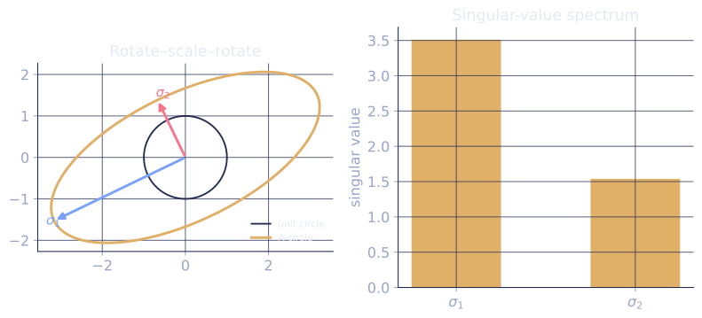
Geometric interpretation

$A = U\Sigma V^\top$ applied to a vector $x$:

1. $V^\top x$: rotate $x$ in the domain $\mathbb{R}^n$.
2. $\Sigma(V^\top x)$: scale the $i$-th coordinate by $\sigma_i$ (and possibly change dimension).
3. $U(\Sigma V^\top x)$: rotate the result in the codomain $\mathbb{R}^m$.

Every linear map is a rotation, followed by axis-aligned scaling, followed by another rotation. The singular values are the scale factors along the principal axes.

The four fundamental subspaces, revisited

From the SVD with $r = \operatorname{rank}(A)$:

• Column space: $\operatorname{span}(u_1, \dots, u_r)$.
• Left null space: $\operatorname{span}(u_{r+1}, \dots, u_m)$.
• Row space: $\operatorname{span}(v_1, \dots, v_r)$.
• Null space: $\operatorname{span}(v_{r+1}, \dots, v_n)$.

These four subspaces are mutually orthogonal in their respective spaces, and their dimensions satisfy rank + nullity = $n$ (rank–nullity theorem confirmed).

Check it on arrays

import numpy as np

A = np.array([[3.0, 2.0, 1.0],
              [0.0, 1.0, 4.0]])   # 2x3 matrix, rank 2

U, s, Vt = np.linalg.svd(A, full_matrices=True)
print("singular values:", np.round(s, 6))
print("U shape:", U.shape, "| Vt shape:", Vt.shape)

# Reconstruct: A = U Sigma V^T
Sigma = np.zeros_like(A)
Sigma[:len(s), :len(s)] = np.diag(s)
A_reconstructed = U @ Sigma @ Vt
print("reconstruction error:", np.max(np.abs(A - A_reconstructed)))   # ~1e-14

# Verify U and V are orthogonal
print("U^T U:\n", np.round(U.T @ U, 10))
print("V^T V:\n", np.round(Vt @ Vt.T, 10))

# Rotate-scale-rotate: trace through on a specific vector
v = np.array([1.0, 0.0, 0.0])
step1 = Vt @ v          # rotate in R^3
step2 = Sigma @ step1   # scale (and reduce to R^2)
step3 = U @ step2       # rotate in R^2
print("A @ v:", A @ v)
print("U Sigma V^T @ v:", np.round(step3, 10))   # same

The reconstruction error is near machine epsilon; both $U$ and $V^\top$ pass the orthogonality check.

Exercises

Exercise 1. Compute the singular values of $A = \begin{bmatrix} 2 & 0 \\ 0 & 3 \\ 0 & 0 \end{bmatrix}$ by hand, using $A^\top A$.

Exercise 2. Show that the nonzero singular values of $A$ equal those of $A^\top$, so $\operatorname{rank}(A) = \operatorname{rank}(A^\top)$.

Exercise 3 (code). For a random $4 \times 3$ matrix, verify that the left singular vectors $u_i = \tfrac{1}{\sigma_i} A v_i$ from the construction match the columns of $U$ that np.linalg.svd returns (up to sign), and that $\lVert A v_i \rVert = \sigma_i$.

import numpy as np

rng = np.random.default_rng(0)
A = rng.normal(size=(4, 3))

U, s, Vt = np.linalg.svd(A, full_matrices=False)
V = Vt.T

for i, sigma in enumerate(s):
    Av = A @ V[:, i]
    u_constructed = Av / sigma
    # ||A v_i|| == sigma_i
    assert np.isclose(np.linalg.norm(Av), sigma)
    # u_constructed equals column i of U up to a sign flip
    assert np.allclose(u_constructed, U[:, i]) or \
           np.allclose(u_constructed, -U[:, i])

print("singular values:", np.round(s, 6))

With the SVD in hand, the next lesson uses it to find the best rank-$k$ approximation to $A$ and to define PCA.

References

- [1]Trefethen, L. N., & Bau, D. (1997). Numerical Linear Algebra. SIAM. Existence and geometry of the SVD (Lectures 4-5).↩
- [2]Golub, G. H., & Van Loan, C. F. (2013). Matrix Computations (4th ed.). Johns Hopkins University Press. The canonical reference for the SVD and its computation (doi:10.56021/9781421407944).↩