Low-rank approximation (Eckart–Young) & PCA

Storing a full $m \times n$ matrix costs $mn$ numbers. Often the matrix is approximately low-rank: most of the information lives in a few directions. The Eckart–Young theorem says the truncated SVD is the optimal compression, and PCA applies this directly to data.

Low-rank approximation

The rank-$k$ truncated SVD of $A = U\Sigma V^\top$ is

using only the $k$ largest singular values and their associated vectors. $A_k$ is a rank-$k$ matrix (a sum of $k$ rank-1 outer products).

Eckart–Young theorem. Among all rank-$k$ matrices $B$[1],

and the same holds with the spectral norm (largest singular value). The truncated SVD is the closest rank-$k$ matrix to $A$ in both the Frobenius and spectral norms.

Proof sketch (Frobenius norm). Write the Frobenius norm using singular values: $\lVert A\rVert_F^2 = \sum_i \sigma_i^2$. The approximation error is

For any rank-$k$ matrix $B$, $B$ has a null space of dimension $\ge n - k$, so there exists a nonzero $w$ in $\operatorname{span}(v_1, \dots, v_{k+1}) \cap \ker B$ (the intersection of a $(k+1)$-dimensional space with the $(n-k)$-dimensional null space of $B$; by dimension count this is at least 1-dimensional). Then

where the last inequality uses the fact that $w$ is in the span of the first $k+1$ right singular vectors and $\lVert Av_{k+1}\rVert = \sigma_{k+1}$. A more careful argument shows the lower bound is $\sum_{i>k}\sigma_i^2$, matching the error of $A_k$. $\qquad\blacksquare$

Energy captured

The fraction of variance explained by $A_k$ is

Plotting this as a function of $k$ gives the scree plot: the knee where adding more components yields diminishing returns is the natural choice of rank.

PCA as truncated SVD

Given a data matrix $X \in \mathbb{R}^{n \times d}$ (rows = samples, columns = features), principal component analysis (PCA) proceeds[2, 3]:

1. Center: subtract the column means, obtaining $\tilde{X}$ with mean zero.
2. Compute SVD: $\tilde{X} = U\Sigma V^\top$.
3. Project onto $k$ components: the score matrix is $Z = \tilde{X} V_k$, where $V_k$ is the first $k$ columns of $V$.

The $i$-th column of $V$ (the $i$-th right singular vector) is the $i$-th principal direction: the direction of maximum remaining variance after removing the previous $i-1$ directions. The corresponding singular value $\sigma_i$ encodes how much variance lies along it ($\sigma_i^2/n$ is the variance in that direction).

The covariance matrix is $\frac{1}{n}\tilde{X}^\top\tilde{X} = \frac{1}{n}V\Sigma^2 V^\top$, so the principal directions are the eigenvectors of the sample covariance and the principal variances are its eigenvalues.

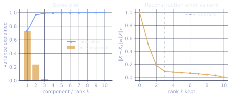
Check it on arrays

import numpy as np

rng = np.random.default_rng(42)

# Synthetic data: 200 samples, 10 features, low-rank signal
d, n, k_true = 10, 200, 3
V_true = np.linalg.qr(rng.normal(size=(d, k_true)))[0]   # 3 orthonormal directions
scores = rng.normal(scale=[5, 3, 1], size=(n, k_true))    # varying variance
X = scores @ V_true.T + 0.2 * rng.normal(size=(n, d))    # signal + noise

# Center
X_c = X - X.mean(axis=0)

# SVD
U, s, Vt = np.linalg.svd(X_c, full_matrices=False)

# Scree: fraction of variance explained
total = (s**2).sum()
explained = np.cumsum(s**2) / total
print("cumulative variance explained (k=1,2,3,4):", np.round(explained[:4], 3))

# Rank-k approximation
k = 3
X_approx = U[:, :k] * s[:k] @ Vt[:k, :]
print(f"rank-{k} Frobenius error / total norm:", np.linalg.norm(X_c - X_approx, 'fro') / np.linalg.norm(X_c, 'fro'))

# PCA scores: project onto first k principal directions
Z = X_c @ Vt[:k].T    # (n, k) scores
print("variance of first component:", np.var(Z[:, 0], ddof=1))
print("expected (s[0]^2 / (n-1)):", s[0]**2 / (n - 1))

The first three components capture most of the variance; the rank-3 approximation has low relative error; and the PCA score variance matches the expected formula.

Exercises

Exercise 1. A matrix has singular values $\sigma = (4, 3, 2, 1)$. Compute the best rank-2 Frobenius approximation error and the fraction of variance explained by the first two components.

Exercise 2. Prove that the rank-$k$ truncated SVD error in Frobenius norm is exactly $\sqrt{\sum_{i>k}\sigma_i^2}$. Use the unitary invariance of the Frobenius norm.

Exercise 3 (code). Generate data along two orthogonal directions with variances 9 and 1 plus small noise. Confirm that PCA recovers the two principal directions (up to sign) and that the first principal variance is near 9.

import numpy as np

rng = np.random.default_rng(7)
n = 4000
d1 = np.array([1.0, 0.0])           # true principal directions
d2 = np.array([0.0, 1.0])
s1 = rng.normal(scale=3.0, size=n)  # variance 9 along d1
s2 = rng.normal(scale=1.0, size=n)  # variance 1 along d2
X = np.outer(s1, d1) + np.outer(s2, d2) + 0.01 * rng.normal(size=(n, 2))

Xc = X - X.mean(axis=0)
U, sv, Vt = np.linalg.svd(Xc, full_matrices=False)

# First principal variance = sigma_1^2 / (n - 1) should be ~ 9.
var1 = sv[0]**2 / (n - 1)
assert abs(var1 - 9.0) < 0.5

# First principal direction aligns with d1 (sign is arbitrary).
assert abs(abs(Vt[0] @ d1) - 1.0) < 1e-2
print("first principal variance:", round(float(var1), 3))

With the best low-rank approximation understood, the next lesson looks at the factorizations that solve linear systems efficiently without forming inverses.

References

- [1]Eckart, C., & Young, G. (1936). "The approximation of one matrix by another of lower rank". Psychometrika, 1, 211-218. doi:10.1007/BF02288367. The original optimality proof for the truncated SVD.↩
- [2]Jolliffe, I. T. (2002). Principal Component Analysis (2nd ed.). Springer. The standard reference for PCA and the variance-maximization view.↩
- [3]Strang, G. (2016). Introduction to Linear Algebra (5th ed.). Wellesley-Cambridge Press. PCA as the SVD of the centered data matrix.↩