Linear maps and matrices

Numbers are not the only things we multiply by scalars and add together; maps between vector spaces can behave the same way. When they do, a single rectangular array of numbers captures everything about them.

What a linear map is

A map $T: V \to W$ is linear if it respects the two vector-space operations:

for all $u, v \in V$ and $\alpha \in \mathbb{R}$. The two conditions collapse into one: $T(\alpha u + \beta v) = \alpha T(u) + \beta T(v)$. A linear map sends linear combinations to linear combinations, with the same coefficients.

Immediate consequences: $T(0) = 0$ (set $\alpha = 0$), and $T(-v) = -T(v)$.

Every linear map is a matrix

Fix bases $\mathcal{B} = \{e_1, \dots, e_n\}$ of $V$ and $\mathcal{C} = \{f_1, \dots, f_m\}$ of $W$. By linearity, knowing $T$ on the basis is enough to know $T$ everywhere: any $v = \sum_j x_j e_j$ gives $T(v) = \sum_j x_j T(e_j)$.

Each $T(e_j)$ is a vector in $W$, so it expands in $\mathcal{C}$: $T(e_j) = \sum_i a_{ij} f_i$. Collect the coefficients into the $m \times n$ matrix $A = [a_{ij}]$. Then for any $v$ with coordinate vector $x \in \mathbb{R}^n$, the coordinate vector of $T(v)$ in $\mathcal{C}$ is $Ax$:

The $j$-th column of $A$ is the coordinate vector of $T(e_j)$.

This is the complete story: a linear map is a matrix, and the matrix depends on the choice of bases[1]. Switch bases and the matrix changes, but it represents the same map.

Composition is matrix multiplication

If $T: U \to V$ has matrix $A$ (in bases $\mathcal{B}, \mathcal{C}$) and $S: V \to W$ has matrix $B$ (in bases $\mathcal{C}, \mathcal{D}$), then the composition $S \circ T: U \to W$ has matrix $BA$.

Proof. For any $u$ with coordinate vector $x$: $(S \circ T)(u) = S(T(u))$. The coordinate vector of $T(u)$ is $Ax$, and then $S$ sends it to $B(Ax) = (BA)x$. So the composite acts as $BA$ on coordinate vectors. $\qquad\blacksquare$

Matrix multiplication is not a formula chosen for convenience; it is the only rule for associating a matrix to a composition of linear maps[2].

The kernel and image

Two subspaces are attached to every linear map:

• Kernel (null space): $\ker T = \{v \in V : T(v) = 0\}$. It is a subspace of $V$ (if $T(u) = T(v) = 0$, then $T(u+v) = 0$ and $T(\alpha u) = 0$).
• Image (column space): $\operatorname{im} T = \{T(v) : v \in V\}$. It is a subspace of $W$.

These are the null space and column space of the matrix $A$ in the chosen bases. The kernel measures how much $T$ collapses, and the image measures how much of $W$ it can reach: two quantifications the rank–nullity theorem connects in the next lesson.

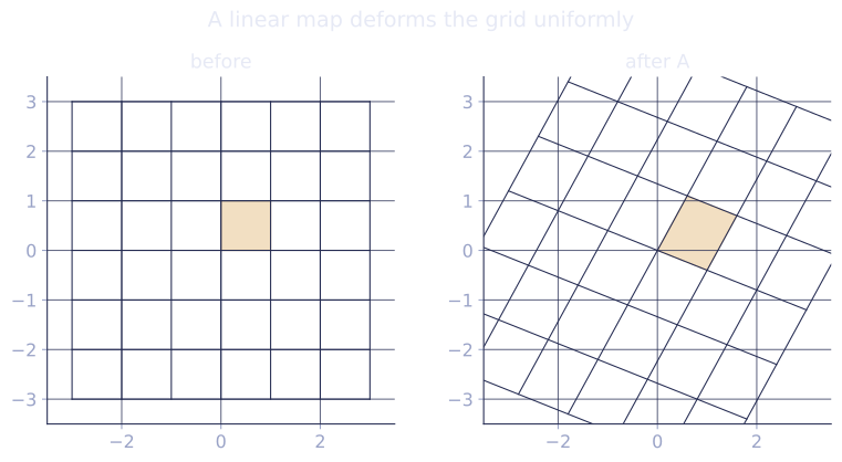
Check it on arrays

The claim is that $T(e_j)$ lands in the $j$-th column of the matrix, and that applying $T$ to a vector is matrix-vector multiplication.

import numpy as np

# Define T: R^3 -> R^2 by its action on the standard basis:
#   T(e1) = [1, 2], T(e2) = [0, -1], T(e3) = [3, 1]
A = np.array([[1.0, 0.0, 3.0],
              [2.0,-1.0, 1.0]])

# v = 2*e1 - e2 + 4*e3
v = np.array([2.0, -1.0, 4.0])
Tv = A @ v
print("T(v):", Tv)   # [1*2+0*(-1)+3*4, 2*2+(-1)*(-1)+1*4] = [14, 9]
print("manual:", 2*A[:,0] - A[:,1] + 4*A[:,2])  # same

# Composition: define S: R^2 -> R^2
B = np.array([[0.0, 1.0],
              [-1.0, 2.0]])

# (S o T)(v) = B @ (A @ v) = (B @ A) @ v
print("B@A@v:", B @ A @ v)
print("B@(A@v):", B @ (A @ v))  # identical

Both routes give the same result, confirming that composition equals matrix multiplication.

Exercises

Exercise 1. A linear map $T: \mathbb{R}^2 \to \mathbb{R}^2$ acts on the standard basis by $T(e_1) = (1, 2)$ and $T(e_2) = (3, -1)$. Write the matrix of $T$ and compute $T(4, 5)$.

Exercise 2. Prove from the linearity axioms that if $v_1, \dots, v_k$ are linearly dependent, then $T(v_1), \dots, T(v_k)$ are linearly dependent. Then give a one-line reason why this forces $\operatorname{rank}(T) \le \dim V$.

Exercise 3 (code). Pick two random matrices $A$ ($4 \times 3$) and $B$ ($2 \times 4$). Verify on a batch of random input vectors that applying the composition $S \circ T$ as $B(Ax)$ equals applying the single matrix $BA$, and that the matrix of the composite is exactly $BA$.

import numpy as np

rng = np.random.default_rng(1)
A = rng.normal(size=(4, 3))   # T: R^3 -> R^4
B = rng.normal(size=(2, 4))   # S: R^4 -> R^2

X = rng.normal(size=(3, 100))         # 100 input vectors as columns
two_step = B @ (A @ X)                 # apply T then S
one_step = (B @ A) @ X                 # apply the composite matrix
assert np.allclose(two_step, one_step)

# The composite's matrix is BA: its j-th column is (S o T)(e_j).
BA = B @ A
for j in range(3):
    e_j = np.zeros(3); e_j[j] = 1.0
    assert np.allclose(B @ (A @ e_j), BA[:, j])
print("composite matrix shape:", BA.shape)

The next lesson asks: given the matrix of $T$, how much of the input does $T$ annihilate, and how much of the output does it fill?

References

- [1]Axler, S. (2015). Linear Algebra Done Right (3rd ed.), ch. 3. Springer. Linear maps and their matrices relative to chosen bases (doi:10.1007/978-3-319-11080-6).↩
- [2]Strang, G. (2016). Introduction to Linear Algebra (5th ed.). Wellesley-Cambridge Press. Matrix multiplication as composition of maps.↩