Inner products, orthogonality, Cauchy–Schwarz

A norm tells you how long a vector is. An inner product tells you how two vectors relate: the angle between them, whether they are perpendicular, how much one points along another. Almost every geometric statement later in the course (projections, least squares, orthogonal attention directions) is an inner-product statement, and they all rest on one inequality we will prove carefully here.

Definition

An inner product on a real vector space $V$ is a rule $\langle u, v\rangle$ assigning a real number to each pair of vectors, with three properties[1]:

1. Symmetry: $\langle u, v\rangle = \langle v, u\rangle$.
2. Linearity in the first slot: $\langle \alpha u + \beta w,\, v\rangle = \alpha\langle u,v\rangle + \beta\langle w,v\rangle$.
3. Positive definiteness: $\langle v, v\rangle \ge 0$, with equality only when $v = 0$.

On $\mathbb{R}^n$ the standard choice is the dot product $\langle u, v\rangle = u^\top v = \sum_i u_i v_i$. Property 3 lets us define a length from the inner product, the induced norm:

For the dot product this is exactly the Euclidean norm from the previous lesson.

The inequality everything depends on

Cauchy–Schwarz inequality. For all $u, v \in V$[2],

with equality if and only if $u$ and $v$ are scalar multiples of each other.

The proof is short once you see the trick: build a quantity that must be nonnegative (a squared length), expand it, and read off the inequality.

Proof. If $v = 0$ both sides are $0$ and the statement holds. So assume $v \neq 0$, and consider the vector $u - t v$ for a real number $t$ we will choose later. By positive definiteness its squared length is nonnegative:

Step 1: start from a square that cannot be negative.

Step 2: expand using symmetry and linearity.

So for every real $t$,

Step 3: a nonnegative quadratic has nonpositive discriminant. The left side is a quadratic $at^2 + bt + c$ in $t$ with $a = \lVert v\rVert^2 > 0$. A parabola that opens upward and never goes below zero can touch zero at most once, which means its discriminant $b^2 - 4ac$ is $\le 0$. Here

Step 4: solve for the inequality. Divide by $4$ and rearrange:

Taking square roots (both sides nonnegative) gives $|\langle u,v\rangle| \le \lVert u\rVert\,\lVert v\rVert$, the claim.

Equality. The discriminant is zero exactly when the quadratic has a real root $t^\star$, i.e. $\lVert u - t^\star v\rVert^2 = 0$, which by positive definiteness forces $u = t^\star v$. So equality holds precisely when $u$ and $v$ are parallel. $\qquad\blacksquare$

Angle and orthogonality

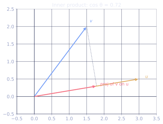
Cauchy–Schwarz says the ratio $\langle u,v\rangle / (\lVert u\rVert\,\lVert v\rVert)$ always lies in $[-1, 1]$. That is exactly the range of cosine, so we may define the angle $\theta$ between two nonzero vectors by

The definition is only legitimate because the inequality guarantees the right-hand side is a valid cosine. The normalized inner product is then an alignment score on a fixed scale from $-1$ to $1$, and the familiar angles sit at recognizable values:

• $\cos\theta = 1$ ($\theta = 0^\circ$): the vectors point the same way, the equality case of Cauchy–Schwarz. $u = (1,0)$ and $v = (3,0)$.
• $\cos\theta = 0.5$ ($\theta = 60^\circ$): $u = (1,0)$ and $v = (1,\sqrt 3)$ give $\langle u,v\rangle = 1$, $\lVert u\rVert = 1$, $\lVert v\rVert = 2$, ratio $0.5$.
• $\cos\theta = 0$ ($\theta = 90^\circ$): perpendicular, $u = (1,0)$ and $v = (0,1)$.
• $\cos\theta = -1$ ($\theta = 180^\circ$): antiparallel, $u = (1,0)$ and $v = (-3,0)$, the other equality case.

Two vectors are orthogonal when $\langle u, v\rangle = 0$, i.e. $\theta = 90^\circ$. This single condition is the seed of projections, the normal equations of least squares, and the orthogonality of principal components later in the course.

A companion fact, proved in one line from the expansion above with $t = -1$, is the triangle inequality for the induced norm: $\lVert u + v\rVert \le \lVert u\rVert + \lVert v\rVert$. So the induced norm is genuinely a norm in the sense of the previous lesson.

Check it on arrays

Cauchy–Schwarz is a claim you can stress-test: for many random pairs the ratio $|\langle u,v\rangle| / (\lVert u\rVert\lVert v\rVert)$ should never exceed $1$, and it should hit $1$ exactly when the two vectors are parallel.

import numpy as np

rng = np.random.default_rng(0)

# 100000 random pairs in R^5: the ratio must stay <= 1.
U = rng.normal(size=(100_000, 5))
V = rng.normal(size=(100_000, 5))
dots = np.einsum("ij,ij->i", U, V)
ratio = np.abs(dots) / (np.linalg.norm(U, axis=1) * np.linalg.norm(V, axis=1))
print("max ratio over 100k random pairs:", ratio.max())   # < 1

# Parallel vectors saturate the bound (ratio == 1):
u = np.array([1.0, 2.0, 3.0])
v = -4.0 * u
print("parallel ratio:", abs(u @ v) / (np.linalg.norm(u) * np.linalg.norm(v)))  # 1.0

# Orthogonal vectors: inner product is 0, angle 90 degrees.
a = np.array([1.0, 0.0]); b = np.array([0.0, 1.0])
print("orthogonal dot:", a @ b, "-> angle", np.degrees(np.arccos(a @ b)))

The random ratios crowd under $1$ but never cross it; the parallel pair sits exactly at $1$ (the equality case of the proof); the orthogonal pair gives $0$.

Exercises

Exercise 1. For $u = (1, 2, 2)$ and $v = (2, 0, 1)$ under the standard dot product, compute $\langle u, v\rangle$, the two norms, and the cosine of the angle between them. Confirm the Cauchy–Schwarz inequality holds.

Exercise 2. Prove the parallelogram law $\lVert u + v\rVert^2 + \lVert u - v\rVert^2 = 2\lVert u\rVert^2 + 2\lVert v\rVert^2$ for any inner-product norm.

Exercise 3 (code). A valid inner product can weight coordinates differently: $\langle u, v\rangle_W = u^\top W v$ for a diagonal $W$ with positive entries. Pick $W = \operatorname{diag}(1, 2, 3)$, draw many random pairs in $\mathbb{R}^3$, and verify Cauchy–Schwarz holds in this weighted inner product (using its induced norm).

import numpy as np

rng = np.random.default_rng(0)
W = np.diag([1.0, 2.0, 3.0])      # positive diagonal -> valid inner product

def ip(u, v):                      # weighted inner product u^T W v
    return u @ W @ v

U = rng.normal(size=(100_000, 3))
V = rng.normal(size=(100_000, 3))

dots = np.einsum("ij,jk,ik->i", U, W, V)        # <u, v>_W per row
nu = np.sqrt(np.einsum("ij,jk,ik->i", U, W, U)) # induced norms
nv = np.sqrt(np.einsum("ij,jk,ik->i", V, W, V))
ratio = np.abs(dots) / (nu * nv)

assert ratio.max() <= 1.0 + 1e-12               # Cauchy-Schwarz, weighted
print("max weighted ratio:", round(ratio.max(), 6))

The next lesson turns orthogonality into a construction, Gram–Schmidt, that manufactures an orthonormal basis from any basis.

References

- [1]Axler, S. (2015). Linear Algebra Done Right (3rd ed.), ch. 6. Springer. Inner-product spaces, orthogonality, and the induced norm (doi:10.1007/978-3-319-11080-6).↩
- [2]Horn, R. A., & Johnson, C. R. (2012). Matrix Analysis (2nd ed.). Cambridge University Press. The Cauchy-Schwarz inequality and its equality conditions.↩