Word embeddings

A neural network cannot consume raw words; it needs vectors. The word embedding is the first deep-learning idea to take over NLP: learn a dense vector for each vocabulary word so that distances in embedding space track semantic similarity. The two recipes that established the field were word2vec (predict context from a word) and GloVe (factorize the global co-occurrence matrix). Both produce embeddings with the same striking property: vector arithmetic captures analogies.

The setup

Build a vocabulary $V$ of words. Assign each word $w \in V$ two $d$-dimensional vectors: an input embedding $u_w$ used when $w$ is the focus word, and an output embedding $v_w$ used when $w$ appears in context. Typical $d$ is 100-300.

The goal: words appearing in similar contexts should have similar embeddings.

word2vec: skip-gram with negative sampling

Mikolov et al. (2013)[1]. Given a center word $w_c$ in a sentence, predict the surrounding context words within a window of size $L$.

Vanilla softmax loss:

The denominator sums over the entire vocabulary, which is enormous ($10^5$ to $10^7$ words). Computing it for every training pair is infeasible.

Negative sampling replaces the softmax with a binary classification: for each true (center, context) pair, sample $k$ random "negative" words and train the model to distinguish positives from negatives.

with $w_i$ sampled from a noise distribution (typically $P(w) \propto f(w)^{3/4}$, where $f(w)$ is unigram frequency).

This makes training $O(k)$ per pair instead of $O(|V|)$ and scales to billions of pairs. Trained on 100B tokens, word2vec produces embeddings that solve the famous analogy "king - man + woman ≈ queen" in vector space.

GloVe: matrix factorization view

Pennington et al. (2014) showed that word2vec is implicitly factorizing a shifted log of the co-occurrence matrix[2]. GloVe does this explicitly:

1. Count $X_{ij}$ = the number of times word $j$ appears in the context of word $i$ across the corpus.
2. Find vectors $u_i, v_j$ and biases $b_i, c_j$ minimizing

where $f$ is a weighting function that downweights very frequent and very rare pairs.

Trained on the same corpus, GloVe produces embeddings of comparable quality to word2vec, slightly faster to train, and with a cleaner mathematical interpretation.

What the embeddings encode

A few invariants that emerged from word2vec / GloVe:

• Semantic similarity: $\cos(u_{\text{king}}, u_{\text{queen}})$ is large.
• Syntactic similarity: $\cos(u_{\text{running}}, u_{\text{jumping}})$ is large.
• Analogies: $u_{\text{king}} - u_{\text{man}} + u_{\text{woman}} \approx u_{\text{queen}}$.
• Polysemy is averaged: "bank" gets one embedding regardless of meaning.

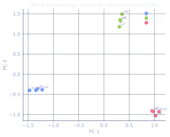
These are not qualitative claims; cosine similarity puts a number on the geometry. The closing code trains skip-gram on a toy corpus and reads off the cosines, which separate cleanly by co-occurrence:

• Two words that share contexts (words 1 and 2 both appear in the sentences [0,1,2,3] and [1,2,7,8]): $\cos = 0.66$. The predictive objective pulled their vectors into near-alignment.
• Two words that never co-occur (words 1 and 9, in disjoint sentences): $\cos = 0.37$. No training signal ever tied them, so they drift toward the random baseline.

That gap, $0.66$ against $0.37$ on the same trained model with the same random initialization, is the whole mechanism in one contrast: the only thing separating the two pairs is whether the words occurred together, and that is what the geometry recovers.

The polysemy limitation is what motivated contextual embeddings (ELMo, BERT): instead of one vector per word, produce a vector per word in context. The next lessons cover the architectures that produce them.

Modern usage

Word2vec / GloVe embeddings are still useful baselines and feature inputs for small models. For state-of-the-art NLP, the embeddings are learned end-to-end inside a Transformer, typically with subword tokenization (Byte-Pair Encoding) so that out-of-vocabulary words are composed from learned pieces.

But the conceptual contribution of word2vec is permanent: distributed representations of discrete symbols, trained by a self-supervised predictive objective, generalizing across NLP, biology (protein embeddings), recommendation systems (item embeddings), and beyond.

Check it on arrays

import numpy as np

rng = np.random.default_rng(0)

# Tiny corpus: each "sentence" is a sequence of word indices
V = 12                                                     # vocab size
sentences = [
    [0, 1, 2, 3], [4, 5, 6], [1, 2, 7, 8], [9, 10, 11],
    [0, 1, 7], [2, 3, 5], [4, 5, 8, 10],
] * 50

# Skip-gram with negative sampling: train embeddings
d = 8
U = rng.normal(scale=0.1, size=(V, d))                     # input embeddings
W = rng.normal(scale=0.1, size=(V, d))                     # output embeddings
window = 2
k_neg = 5

def sigmoid(z): return 1 / (1 + np.exp(-z))

for epoch in range(50):
    for sent in sentences:
        for i, c in enumerate(sent):                       # center
            for j in range(max(0, i - window), min(len(sent), i + window + 1)):
                if j == i: continue
                o = sent[j]                                # positive context
                # Positive pair
                p_pos = sigmoid(U[c] @ W[o])
                grad_c = (p_pos - 1) * W[o]
                grad_o = (p_pos - 1) * U[c]
                U[c] -= 0.1 * grad_c
                W[o] -= 0.1 * grad_o
                # Negative samples (exclude the positive context and the center)
                for _ in range(k_neg):
                    n = int(rng.integers(0, V))
                    while n == o or n == c:
                        n = int(rng.integers(0, V))
                    p_neg = sigmoid(U[c] @ W[n])
                    grad_c = p_neg * W[n]                  # compute both grads BEFORE either update
                    grad_n = p_neg * U[c]
                    U[c] -= 0.1 * grad_c
                    W[n] -= 0.1 * grad_n

# Cosine similarity between learned embeddings
def cos(u, v): return u @ v / (np.linalg.norm(u) * np.linalg.norm(v) + 1e-12)
print("similarity(word 1, word 2) =", round(cos(U[1], U[2]), 3),
      "(both appear in sentences [0,1,2,3] and [1,2,7,8])")
print("similarity(word 1, word 9) =", round(cos(U[1], U[9]), 3),
      "(word 1 and word 9 never co-occur)")

Words that co-occur in the toy corpus learn similar embeddings; words that never co-occur do not.

Exercises

Exercise 1. A skip-gram model has center vector $u_c = (1, 0)$ and a true context vector $v_o = (2, 1)$. Compute the positive-pair loss $-\log \sigma(u_c^\top v_o)$ and the gradient $\partial \mathcal{L} / \partial u_c = (\sigma(u_c^\top v_o) - 1)\, v_o$ by hand. Use $\sigma(2) \approx 0.8808$ and $\ln(0.8808) \approx -0.1269$.

Exercise 2. GloVe weights its squared error by $f(X_{ij})$. The standard choice is $f(x) = (x / x_{\max})^\alpha$ for $x < x_{\max}$ and $f(x) = 1$ otherwise, with $\alpha = 3/4$ and $x_{\max} = 100$. Compute $f(1)$, $f(10)$, and $f(100)$, and explain in one line what the weighting buys.

Exercise 3 (code). Verify on the trained toy embeddings that the skip-gram objective separates co-occurring words from non-co-occurring words: the mean cosine similarity over pairs that share a sentence should exceed the mean over pairs that never share one.

import numpy as np

rng = np.random.default_rng(0)

V = 12
sentences = [
    [0, 1, 2, 3], [4, 5, 6], [1, 2, 7, 8], [9, 10, 11],
    [0, 1, 7], [2, 3, 5], [4, 5, 8, 10],
] * 50

d = 8
U = rng.normal(scale=0.1, size=(V, d))
W = rng.normal(scale=0.1, size=(V, d))
window, k_neg = 2, 5

def sigmoid(z): return 1 / (1 + np.exp(-z))

for epoch in range(50):
    for sent in sentences:
        for i, c in enumerate(sent):
            for j in range(max(0, i - window), min(len(sent), i + window + 1)):
                if j == i: continue
                o = sent[j]
                p_pos = sigmoid(U[c] @ W[o])
                gc, go = (p_pos - 1) * W[o], (p_pos - 1) * U[c]
                U[c] -= 0.1 * gc; W[o] -= 0.1 * go
                for _ in range(k_neg):
                    n = int(rng.integers(0, V))
                    while n == o or n == c:
                        n = int(rng.integers(0, V))
                    p_neg = sigmoid(U[c] @ W[n])
                    gc, gn = p_neg * W[n], p_neg * U[c]
                    U[c] -= 0.1 * gc; W[n] -= 0.1 * gn

def cos(a, b): return a @ b / (np.linalg.norm(a) * np.linalg.norm(b) + 1e-12)

# Build the set of unordered pairs that share at least one sentence
cooccur = set()
for sent in sentences:
    for a in sent:
        for b in sent:
            if a < b: cooccur.add((a, b))

co_sims, non_sims = [], []
for a in range(V):
    for b in range(a + 1, V):
        s = cos(U[a], U[b])
        (co_sims if (a, b) in cooccur else non_sims).append(s)

mean_co = np.mean(co_sims)
mean_non = np.mean(non_sims)
assert mean_co > mean_non
print("mean cosine, co-occurring pairs:    ", round(mean_co, 3))
print("mean cosine, non-co-occurring pairs:", round(mean_non, 3))

The next lesson tackles sequences directly with recurrent networks.

References

- [1]Mikolov, T., Chen, K., Corrado, G., & Dean, J. (2013). "Efficient estimation of word representations in vector space (word2vec)". arXiv:1301.3781. Introduces skip-gram and CBOW with negative sampling.↩
- [2]Pennington, J., Socher, R., & Manning, C. D. (2014). "GloVe: global vectors for word representation". EMNLP. doi:10.3115/v1/D14-1162. The global co-occurrence matrix-factorization view of embeddings.↩