Linear and sub-quadratic attention

The Transformer's quadratic cost in sequence length is the headline bottleneck. Two lines of work attack it: algorithmic approaches that approximate or restructure attention to be sub-quadratic, and systems approaches that keep exact attention but make it hardware-efficient. Both are now standard parts of large-scale training, and modern long-context models combine them with the SSM methods from the previous lesson.

The cost to attack

Standard attention computes $\operatorname{softmax}(QK^\top/\sqrt{d})V$[2]:

• $QK^\top$: $O(N^2 d)$ FLOPs, materializes an $N \times N$ matrix.
• $\operatorname{softmax}$: $O(N^2)$ FLOPs, requires the full matrix.
• $A V$: $O(N^2 d)$ FLOPs.

Memory is $O(N^2)$ for the attention matrix at training time. At $N = 100\text{K}$, that is 10 GB just for one attention layer's intermediate.

Linformer: low-rank approximation

Wang et al. (2020). Project the keys and values to a small fixed dimension $k \ll N$ before computing attention:

$$K' = E K \in \mathbb{R}^{k \times d}, \qquad V' = F V \in \mathbb{R}^{k \times d}.$$

Attention is then $\operatorname{softmax}(Q K'^\top / \sqrt{d}) V'$ with size $N \times k$, which is $O(Nkd)$ cost: linear in $N$ for fixed $k$.

Simple, works reasonably, but the low-rank assumption is empirical and may not hold for all input distributions.

Performer / Linear Attention: kernel feature map

Choromanski et al. (2021). Replace softmax with a kernel:

$$\operatorname{softmax}(q^\top k) \approx \phi(q)^\top \phi(k),$$

with $\phi: \mathbb{R}^d \to \mathbb{R}^m$ a random feature map. Then attention rewrites:

$$A V = \phi(Q)\,\phi(K)^\top\, V = \phi(Q)\,(\phi(K)^\top V).$$

Compute $\phi(K)^\top V \in \mathbb{R}^{m \times d}$ first ($O(N m d)$ cost), then multiply by $\phi(Q)$ ($O(N m d)$ cost). Total cost $O(Nmd)$ instead of $O(N^2 d)$. Reordering the products this way also exposes an exact recurrent form, making a linear-attention layer an RNN at inference time[1].

Performers use random features that approximate the softmax kernel unbiased. Other "linear attention" variants use elu+1, ReLU, or other kernels.

Practical quality on language modeling: 1-2 perplexity worse than full attention at the same parameter count, but the linear scaling lets you trade those points for longer context or more parameters.

Sparse attention

Restrict attention to a sparse pattern instead of all $N \times N$:

• Local attention: each token attends only to the $w$ nearest neighbors. $O(Nw)$ cost.
• Strided attention: attend to every $k$-th token plus a local window. Used in Sparse Transformer.
• Global tokens: a few special tokens attend to everything; everyone attends to them; otherwise local.

Longformer and BigBird combine local + global + random patterns to achieve linear cost with provable expressiveness.

FlashAttention: exact, IO-aware

Dao et al. (2022). Keep the exact softmax-attention computation, but implement it as a fused CUDA kernel that tiles the computation into chunks fitting in fast GPU SRAM:

1. Split $Q$, $K$, $V$ into blocks.
2. For each block of $Q$, iterate over blocks of $K$ and $V$, incrementally computing the softmax via online running statistics.
3. Never materialize the full $N \times N$ attention matrix in HBM (slow GPU memory); keep it in SRAM (fast).

Result: 2-4x faster than the standard implementation, $O(N)$ memory instead of $O(N^2)$ for the intermediate matrix.

FlashAttention is now the default in every production Transformer training pipeline. FlashAttention-2 further improves parallelism; FlashAttention-3 uses NVIDIA Hopper-specific instructions for another 1.5-2x speedup.

The key insight: attention is bottlenecked by memory bandwidth, not FLOPs. FlashAttention does the same FLOPs but moves much less data between memory tiers.

Approximate vs exact

Linear-attention methods make the FLOPs cheaper at some accuracy cost; FlashAttention makes the same exact computation faster by being kinder to the memory hierarchy.

For most production use cases as of 2024:

• FlashAttention is the no-brainer baseline.
• Linear / sparse attention is used when context length is so long ($>100\text{K}$ tokens) that even FlashAttention is too expensive.
• SSMs and hybrids (next lesson) compete with all of the above for long-context modeling.

The KV-cache angle

At inference, attention's quadratic cost shows up differently: the KV cache stores keys and values for all preceding tokens, growing linearly with context length. Each generated token requires attention against the full cache, so per-token inference is $O(N)$ even with linear-attention or FlashAttention.

For 1M-token contexts, the KV cache alone is gigabytes. Solutions:

• Multi-query attention (MQA) and grouped-query attention (GQA): share keys and values across heads, reducing cache size by factors of 8-64.
• Paged attention (vLLM): page the KV cache like virtual memory.
• SSMs: constant cache size regardless of context.

Exercises

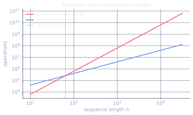
Exercise 1. Linear attention replaces $\operatorname{softmax}(q^\top k)$ with a kernel feature map $\phi(q)^\top \phi(k)$, so that $AV = \phi(Q)\,(\phi(K)^\top V)$. Count the FLOPs of computing the output two ways for $N$ tokens, feature dimension $m$, and value dimension $d$: (a) left-to-right as $(\phi(Q)\phi(K)^\top)V$, and (b) right-to-left as $\phi(Q)(\phi(K)^\top V)$. State the crossover that makes (b) the win.

Solution

Step 1. Left-to-right. First form $S = \phi(Q)\phi(K)^\top$, an $N \times N$ matrix: each of its $N^2$ entries is an inner product of length $m$, so $O(N^2 m)$ FLOPs and $O(N^2)$ memory. Then $S V$ costs $O(N^2 d)$. Total $O(N^2(m + d))$, quadratic in $N$.

Step 2. Right-to-left. First form $T = \phi(K)^\top V$, an $m \times d$ matrix: a sum over the $N$ tokens of outer products, $O(N m d)$ FLOPs and only $O(md)$ memory. Then $\phi(Q) T$ costs $O(N m d)$. Total $O(N m d)$, linear in $N$.

Step 3. Associativity of matrix multiplication makes the two outputs identical, so the only difference is cost. Right-to-left wins whenever $N m d \ll N^2(m+d)$, i.e. roughly when $m \ll N$: once the feature dimension is much smaller than the sequence length, reordering turns a quadratic cost into a linear one. The same reordering also collapses the $N \times N$ intermediate, removing the $O(N^2)$ memory.

Exercise 2. The right-to-left grouping $\phi(Q)(\phi(K)^\top V)$ exposes a recurrence that makes a linear-attention layer an RNN at inference. Define $S_t = \sum_{i \le t} \phi(k_i) v_i^\top$ for causal attention and write the per-step update and output. Compare its per-token inference cost and memory with the KV cache of softmax attention.

Solution

Step 1. For causal attention the (unnormalized) output at position $t$ sums only over $i \le t$:

$$o_t = \phi(q_t)^\top \sum_{i \le t} \phi(k_i) v_i^\top = \phi(q_t)^\top S_t, \qquad S_t = \sum_{i \le t} \phi(k_i) v_i^\top.$$

Step 2. $S_t$ obeys a rank-one recurrence:

$$S_t = S_{t-1} + \phi(k_t)\, v_t^\top,$$

a running sum updated by one outer product per step. The state $S_t \in \mathbb{R}^{m \times d}$ has fixed size $md$, independent of $t$. Each step costs $O(md)$ for the update plus $O(md)$ for $\phi(q_t)^\top S_t$.

Step 3. So linear attention generates with $O(md)$ time and $O(md)$ memory per token, both constant in the context length. Softmax attention instead stores a KV cache that grows to length $t$, costing $O(td)$ time and $O(td)$ memory at step $t$. The constant-size state is exactly the "transformers are RNNs" result: the linear-attention layer carries a fixed recurrent state rather than an unbounded cache.

Exercise 3. Three methods cut attention's cost differently: Linformer projects $K, V$ to a fixed rank $k$, Performer uses an $m$-dimensional random feature map, and FlashAttention keeps the exact softmax but tiles the computation. Classify each as approximate or exact, give its asymptotic time and memory in $N$, and explain why FlashAttention does not reduce per-token inference cost against a KV cache even though it reduces training memory.

Solution

Step 1. Linformer: approximate (the low-rank projection $K' = EK$ discards information when the true attention matrix is not rank-$k$). Cost $O(Nkd)$ time, $O(Nk)$ memory: linear in $N$ for fixed $k$.

Step 2. Performer: approximate (random features estimate the softmax kernel with variance that vanishes only as $m \to \infty$). Cost $O(Nmd)$ time, $O(md + Nd)$ memory: linear in $N$.

Step 3. FlashAttention: exact (it computes the same softmax attention, only reordering the arithmetic with online softmax statistics). Training cost $O(N^2 d)$ FLOPs, but memory $O(N)$ instead of $O(N^2)$ because the $N \times N$ matrix is never materialized in slow memory.

Step 4. At inference with a KV cache, generation is one token at a time and each new token still attends against all $N$ cached keys, an $O(N)$ exact computation. FlashAttention reduces the constant (less data moved between memory tiers) but not the order: it does the same FLOPs, so the per-token cost stays $O(N)$. Only an approximate method (linear/sparse) or a recurrent replacement (SSM, linear attention) changes that asymptotic.

The big picture

The Transformer's quadratic attention has been attacked from every angle: lower-rank approximations, sparse patterns, kernel features, memory-aware kernels, and complete architectural replacements. The next lesson covers the synthesis: hybrid architectures that combine the strengths of multiple sequence-mixing operations.

---

References

1. [1]Katharopoulos, A., Vyas, A., Pappas, N., & Fleuret, F. (2020). "Transformers are RNNs: fast autoregressive transformers with linear attention". ICML. arXiv:2006.16236. Replaces the softmax with a kernel feature map for linear-time attention.↩
2. [2]Vaswani, A., et al. (2017). "Attention is all you need". NeurIPS. arXiv:1706.03762. The exact softmax attention whose quadratic cost these methods attack.↩