Self-attention

The single operation behind the Transformer revolution: self-attention[1]. Each token in a sequence computes a query, a key, and a value; the attention from token $i$ to token $j$ is the (scaled, softmaxed) inner product of $i$'s query with $j$'s key, used to weight $j$'s value into $i$'s output. Three projections, one softmax: content-based mixing across arbitrary positions in one parallel operation.

The operation

Given a sequence of $N$ token embeddings stacked as $X \in \mathbb{R}^{N \times d}$:

1. Project each token to a query, key, and value with learned matrices $W_Q, W_K, W_V \in \mathbb{R}^{d \times d_k}$: $$Q = X W_Q, \quad K = X W_K, \quad V = X W_V.$$
2. Compute the attention scores as scaled dot products: $$S = \frac{Q K^\top}{\sqrt{d_k}}.$$
3. Apply softmax row-wise to get attention weights: $$A = \operatorname{softmax}_{\text{row}}(S).$$
4. The output is the weighted sum of values: $$Y = A V.$$

The output $Y \in \mathbb{R}^{N \times d_k}$ has one row per token, each a content-based mixture of the values of every other token.

What each piece does

• Query: "what am I looking for?" Each token's query interrogates the rest of the sequence.
• Key: "what do I offer?" Each token's key says what it can answer.
• Value: "what do I contribute?" Each token's value is what gets mixed in if it is attended to.

The softmax row $A_{i, :}$ is a probability distribution over the sequence, specifying how much token $i$ attends to each other token.

The $\sqrt{d_k}$ scaling

Without scaling, the dot product $q^\top k$ has variance $d_k$ when $q, k$ are unit-variance Gaussians. Large $d_k$ pushes the softmax into the saturated regime where one entry dominates and gradients vanish. Dividing by $\sqrt{d_k}$ keeps the variance constant in $d_k$, preserving useful attention distributions.

Concretely, take $d_k = 64$ (a standard head size) and one query against $10$ keys, all unit-variance Gaussian. The raw scores then have standard deviation $\sqrt{64} = 8$, so the largest is typically several units above the rest, and the softmax collapses onto it: averaged over random draws, the top weight sits at about $0.86$ of the total mass, nearly a hard argmax over $10$ positions. Divide by $\sqrt{d_k} = 8$ and the scores have unit spread; the top weight drops to about $0.32$, a distribution that still spreads attention and still has gradient. The scaling is the difference between a soft lookup and a saturated one-hot.

Why it works

Self-attention has three properties that make it dominant for sequences:

• Content-based addressing: tokens find their relevant neighbors by similarity, not position. A token can attend to anything anywhere.
• Parallel over positions: all $N$ outputs are computed simultaneously, unlike RNNs which serialize through time. GPU-friendly.
• Constant path length: any pair of tokens is exactly one operation away from influencing each other, no matter how far apart they are in the sequence. RNNs have $O(N)$ path length; self-attention has $O(1)$.

The cost: quadratic in sequence length. Computing $QK^\top$ is $O(N^2 d_k)$ time and $O(N^2)$ memory. For long sequences (1k, 100k, 1M tokens) this becomes the bottleneck, motivating the linear-attention and SSM lessons later.

Multi-head attention

A single attention computation uses one fixed $d_k$. Multi-head attention runs $H$ parallel attentions on different $d_k$-dimensional projections of the input, then concatenates their outputs:

where each $\text{head}_h = \text{Attention}(X W_Q^h, X W_K^h, X W_V^h)$ and $W_O \in \mathbb{R}^{H d_k \times d}$ is a learned output projection.

With $H = 8$ heads and $d_k = d/H = 64$ (for $d = 512$), each head can specialize: one head might attend to syntactic neighbors, another to semantic similarity, another to positional patterns. Empirically heads specialize without being told to.

Masking

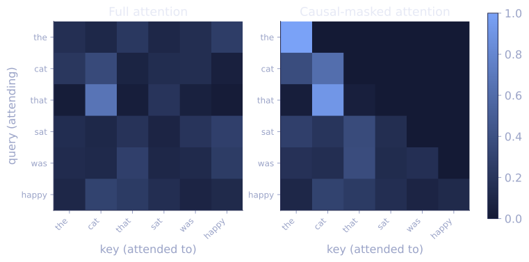
For autoregressive language modeling, the decoder must not see future tokens. Apply a causal mask to the attention scores:

After softmax, $A_{i, j} = 0$ for $j > i$. Token $i$ only attends to tokens at positions $\le i$.

For variable-length sequences in a batch, a padding mask is also applied so padded positions get $-\infty$ scores.

Self-attention vs cross-attention

• Self-attention: $Q$, $K$, $V$ all come from the same sequence. Used in encoder layers and self-attention sublayers of decoder layers.
• Cross-attention: $Q$ comes from the decoder, $K$ and $V$ come from the encoder. The decoder queries the encoder's representation. Used in encoder-decoder Transformers (translation, summarization). This is the direct successor of seq2seq attention[2].

The next lesson assembles these primitives into the full Transformer.

Check it on arrays

import numpy as np

rng = np.random.default_rng(0)

def softmax(z, axis):
    z = z - z.max(axis=axis, keepdims=True)
    e = np.exp(z); return e / e.sum(axis=axis, keepdims=True)

def attention(Q, K, V, mask=None):
    d_k = Q.shape[-1]
    S = Q @ K.T / np.sqrt(d_k)
    if mask is not None:
        S = np.where(mask, S, -np.inf)
    A = softmax(S, axis=-1)
    return A @ V, A

# 5-token sequence, model dim 8
N, d, d_k = 5, 8, 8
X = rng.normal(size=(N, d))
W_q = rng.normal(scale=0.3, size=(d, d_k))
W_k = rng.normal(scale=0.3, size=(d, d_k))
W_v = rng.normal(scale=0.3, size=(d, d_k))

Q = X @ W_q; K = X @ W_k; V = X @ W_v
Y, A = attention(Q, K, V)
print(f"attention matrix shape: {A.shape}, output shape: {Y.shape}")
print(f"each row of A sums to 1: {[round(a, 3) for a in A.sum(axis=1)]}")

# Causal mask: lower-triangular ones
causal = np.tril(np.ones((N, N))).astype(bool)
Y_c, A_c = attention(Q, K, V, mask=causal)
print(f"\ncausal attention matrix (row i can only see j <= i):")
print(A_c.round(2))
print(f"row 2 mass on positions > 2: {A_c[2, 3:].sum():.6f}  (should be 0)")

# Multi-head: 4 heads, each with d_k = d / 4 = 2
H = 4; d_k = d // H
W_qm = rng.normal(scale=0.3, size=(H, d, d_k))
W_km = rng.normal(scale=0.3, size=(H, d, d_k))
W_vm = rng.normal(scale=0.3, size=(H, d, d_k))
W_o = rng.normal(scale=0.3, size=(H * d_k, d))

heads = []
for h in range(H):
    Qh = X @ W_qm[h]; Kh = X @ W_km[h]; Vh = X @ W_vm[h]
    Yh, _ = attention(Qh, Kh, Vh)
    heads.append(Yh)
Y_multi = np.concatenate(heads, axis=-1) @ W_o
print(f"\nmulti-head output shape: {Y_multi.shape}")

The attention matrix is row-stochastic, the causal mask zeroes out future positions, and the multi-head computation returns to the original embedding dimension.

Exercises

Exercise 1. A single query $q = (1, 0)$ attends to two keys $k_1 = (1, 0)$ and $k_2 = (0, 1)$, with $d_k = 2$ and values $v_1 = (4, 0)$, $v_2 = (0, 4)$. Compute the scaled scores, the softmax attention weights, and the output by hand. Use $e^{1/\sqrt{2}} \approx 2.0281$ and $\sqrt{2} \approx 1.4142$.

Exercise 2. Without scaling, $q^\top k$ for unit-variance Gaussian $q, k \in \mathbb{R}^{d_k}$ has variance $d_k$. Show this, and state what dividing by $\sqrt{d_k}$ does to the variance.

Exercise 3 (code). Confirm the variance argument of Exercise 2 empirically, and show that the unscaled softmax saturates while the scaled one stays soft. Sample many random $(q, k)$ pairs at $d_k = 64$, measure the variance of $q^\top k$ with and without scaling, and compare the average top softmax weight over $10$ keys.

import numpy as np

rng = np.random.default_rng(0)
d_k, n_keys, trials = 64, 10, 20000

def softmax(z):
    z = z - z.max(axis=-1, keepdims=True)
    e = np.exp(z)
    return e / e.sum(axis=-1, keepdims=True)

# Variance of q . k with and without the 1/sqrt(d_k) scaling
q = rng.normal(size=(trials, d_k))
k = rng.normal(size=(trials, d_k))
dots = np.sum(q * k, axis=1)
var_unscaled = dots.var()
var_scaled = (dots / np.sqrt(d_k)).var()
assert np.isclose(var_unscaled, d_k, rtol=0.05)   # variance ~ d_k
assert np.isclose(var_scaled, 1.0, rtol=0.05)     # scaling -> variance ~ 1

# Top softmax weight over n_keys keys, unscaled vs scaled
q1 = rng.normal(size=(trials, d_k))
K = rng.normal(size=(trials, n_keys, d_k))
scores = np.einsum("td,tkd->tk", q1, K)
top_unscaled = softmax(scores).max(axis=1).mean()
top_scaled = softmax(scores / np.sqrt(d_k)).max(axis=1).mean()
assert top_unscaled > top_scaled                  # unscaled saturates harder
print("var unscaled:", round(var_unscaled, 1), " var scaled:", round(var_scaled, 3))
print("mean top weight  unscaled:", round(top_unscaled, 3),
      " scaled:", round(top_scaled, 3))

The next lesson stacks attention and FFN blocks into the full Transformer.

References

- [1]Vaswani, A., et al. (2017). "Attention is all you need". NeurIPS. arXiv:1706.03762. Defines scaled dot-product and multi-head self-attention.↩
- [2]Bahdanau, D., Cho, K., & Bengio, Y. (2015). "Neural machine translation by jointly learning to align and translate". ICLR. arXiv:1409.0473. The encoder-decoder attention that cross-attention generalizes.↩