Recurrent networks

A feed-forward network has no notion of time. To process sequences, recurrent neural networks (RNNs) carry a hidden state from one timestep to the next, so the prediction at time $t$ depends on every input from time 1 to $t$. The vanilla RNN is conceptually clean but trains poorly on long sequences; the next lesson's gated variants fix this.

The RNN cell

At each timestep $t$, the RNN consumes input $x_t \in \mathbb{R}^{d_{\text{in}}}$ and the previous hidden state $h_{t-1} \in \mathbb{R}^{d_h}$, and produces a new hidden state and an output:

The same parameters $W_x, W_h, W_y, b, c$ are used at every timestep. This weight sharing across time is what makes the network handle sequences of arbitrary length with a fixed parameter count.

Unrolling through time

To train, "unroll" the recurrence into a $T$-layer feed-forward network where layer $t$ has the same weights as every other layer:

Compute the loss $\mathcal{L}$ as a function of all $y_t$ (or just $y_T$, depending on the task), then backprop through the entire unrolled graph. This is backpropagation through time (BPTT).

The gradients with respect to a single weight matrix $W_h$ sum contributions from every timestep:

Vanishing and exploding gradients

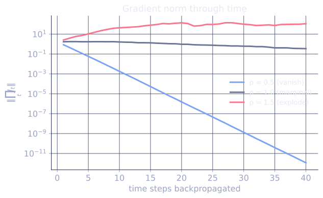
The bad news. The gradient at an early timestep $t$ is a product of $T - t$ recurrence Jacobians:

Each factor is the Jacobian of one tanh step: $\operatorname{diag}(1 - \tanh^2)\cdot W_h$. The product is well-behaved only if its eigenvalues stay near 1; in practice they do not:

• Vanishing: if the spectral radius is below 1, the product shrinks exponentially. Gradients from far in the past die before reaching current weights. The network cannot learn long-range dependencies.
• Exploding: if the spectral radius is above 1, the product grows exponentially. Single gradient updates become huge, training NaNs.

Both regimes are easy to enter[1]. Vanilla RNNs in practice learn dependencies of length 10-20; longer ranges require the gated variants of the next lesson[2].

Gradient clipping

A practical bandage for exploding gradients: cap the global gradient norm:

Standard in RNN training (and still useful in Transformers). Clipping does not fix vanishing gradients; for that, the architecture itself must change.

When RNNs are still used

The dominant sequence architecture for years (2014-2018), then largely replaced by Transformers and state space models[3]. Still useful when:

• Memory matters: an RNN processes sequences of arbitrary length with constant memory per step.
• Streaming: producing output as input arrives, without buffering.
• Very long context where attention is infeasible: SSMs (D3 lesson) are also good here.
• Small models for edge / mobile inference.

For language modeling at scale, Transformers and SSM hybrids dominate. For control / RL with sequential state, RNN-style updates are still common.

Variants beyond LSTM/GRU

• Bidirectional RNN: stack a forward-time RNN and a backward-time RNN; concatenate the hidden states. Standard for encoders that can see the whole input (text classification, sequence labeling).
• Stacked RNN: multiple RNN layers on top of each other, each consuming the previous layer's outputs as inputs. Like deep MLP stacking, gives a more expressive function class.

The next lesson tackles the vanishing-gradient problem head-on with LSTM and GRU gates.

Check it on arrays

import numpy as np

rng = np.random.default_rng(0)

def rnn_forward(X, Wx, Wh, b):
    """X: (T, d_in). Returns (T, d_h) hidden state sequence."""
    T = len(X); d_h = Wh.shape[0]
    H = np.zeros((T, d_h))
    h = np.zeros(d_h)
    for t in range(T):
        h = np.tanh(Wx @ X[t] + Wh @ h + b)
        H[t] = h
    return H

T, d_in, d_h = 30, 5, 8
X = rng.normal(size=(T, d_in))
Wx = rng.normal(scale=0.3, size=(d_h, d_in))
Wh = rng.normal(scale=0.3, size=(d_h, d_h))
b = np.zeros(d_h)

H = rnn_forward(X, Wx, Wh, b)
print(f"hidden state shape: {H.shape}")
print(f"hidden state norm over time: {[round(np.linalg.norm(H[t]), 2) for t in range(0, T, 5)]}")

# Demonstrate vanishing gradient: compute |dh_T / dh_t| as t decreases
def jacobian_product_norm(Wh, H, target):
    """Product of one-step Jacobians dh_{k+1}/dh_k = diag(1 - tanh^2(...)) @ Wh."""
    J = np.eye(Wh.shape[0])
    for k in range(target, len(H) - 1):
        D = np.diag(1 - H[k]**2)
        J = (D @ Wh) @ J
    return np.linalg.norm(J)

# Use a Wh with spectral radius ~ 0.5 (typical for stable training): vanishing.
# An iid Gaussian matrix with std sigma has spectral radius ~ sigma * sqrt(d_h)
# (circular law), so we scale by 1/sqrt(d_h) to control the radius directly.
Wh_small = (0.5 / np.sqrt(d_h)) * rng.normal(size=(d_h, d_h))
H_small = rnn_forward(X, Wx, Wh_small, b)
norms_small = [jacobian_product_norm(Wh_small, H_small, t) for t in range(T - 1, -1, -5)]
print(f"\nvanishing: ||dh_T/dh_t|| from late to early steps: "
      f"{[round(n, 3) for n in norms_small]}")

# Use a Wh with spectral radius ~ 1.5: exploding
Wh_big = (1.5 / np.sqrt(d_h)) * rng.normal(size=(d_h, d_h))
H_big = rnn_forward(X, Wx, Wh_big, b)
norms_big = [jacobian_product_norm(Wh_big, H_big, t) for t in range(T - 1, -1, -5)]
print(f"exploding: ||dh_T/dh_t|| from late to early steps: "
      f"{[round(n, 1) for n in norms_big]}")

The Jacobian product shrinks geometrically with small weights and grows geometrically with large weights, visible across just 30 timesteps.

Exercises

Exercise 1. A scalar RNN has $h_t = \tanh(w_x x_t + w_h h_{t-1} + b)$ with $w_x = 0.5$, $w_h = 1.0$, $b = 0$, and $h_0 = 0$. Compute $h_1$ and $h_2$ by hand for the input sequence $x_1 = 2$, $x_2 = -1$. Use $\tanh(1) \approx 0.7616$ and $\tanh(0.2616) \approx 0.2558$.

Exercise 2. The one-step recurrence Jacobian is $J_t = \operatorname{diag}(1 - \tanh^2(\cdot))\, W_h$. Suppose every tanh saturates so $1 - \tanh^2 = 0.25$ at every unit, and $W_h$ has spectral norm $\lVert W_h \rVert_2 = 2$. Bound the norm of the product $\partial h_T / \partial h_t$ over $T - t = 20$ steps, and say whether it vanishes or explodes.

Exercise 3 (code). Implement scalar BPTT for the recurrence of Exercise 1 and verify the analytic gradient $\partial h_2 / \partial w_h$ against a finite-difference estimate. With $h_0 = 0$, the only $h_{t-1}$-dependence comes through $h_1$, so $\partial h_2 / \partial w_h = (1 - h_2^2)\,[\,h_1 + w_h (1 - h_1^2) h_0\,] = (1 - h_2^2)\, h_1$.

import numpy as np

wx, wh, b = 0.5, 1.0, 0.0
x1, x2 = 2.0, -1.0
h0 = 0.0

def h2_of(wh):
    h1 = np.tanh(wx * x1 + wh * h0 + b)
    h2 = np.tanh(wx * x2 + wh * h1 + b)
    return h2, h1

h2, h1 = h2_of(wh)

# Analytic: chain rule through h1, with h0 = 0 killing the h0 branch
analytic = (1 - h2**2) * (h1 + wh * (1 - h1**2) * h0)

# Finite difference
eps = 1e-6
num = (h2_of(wh + eps)[0] - h2_of(wh - eps)[0]) / (2 * eps)

assert np.isclose(analytic, num, atol=1e-6)
print("h1 =", round(h1, 4), " h2 =", round(h2, 4))
print("analytic dh2/dwh =", round(analytic, 6), " numeric =", round(num, 6))

The next lesson fixes the problem at the architectural level: LSTM and GRU.

References

- [1]Goodfellow, I., Bengio, Y., & Courville, A. (2016). Deep Learning, §10.7 (The Challenge of Long-Term Dependencies). MIT Press. The vanishing/exploding gradient analysis for recurrent nets.↩
- [2]Hochreiter, S., & Schmidhuber, J. (1997). "Long short-term memory". Neural Computation, 9(8), 1735-1780. doi:10.1162/neco.1997.9.8.1735. The gated cell that fixes vanishing gradients.↩
- [3]Sutskever, I., Vinyals, O., & Le, Q. V. (2014). "Sequence to sequence learning with neural networks". NeurIPS. arXiv:1409.3215. LSTM encoder-decoders as the dominant sequence architecture of the era.↩