LSTM and GRU

The vanilla RNN's vanishing gradient comes from repeatedly multiplying small numbers through long products. LSTM and GRU introduce gates that let information flow through time unmultiplied by the recurrence Jacobian. The result: long-range dependencies become trainable, and RNNs dominated sequence modeling for nearly a decade.

LSTM (Long Short-Term Memory)

Hochreiter and Schmidhuber (1997)[1]. Maintain two states per timestep: the cell state $c_t$ (the long-term memory) and the hidden state $h_t$ (the output). Four gates control how the cell state updates.

Given input $x_t$ and previous states $(h_{t-1}, c_{t-1})$:

Gates (each is a sigmoid-activated linear function):

Candidate new memory (tanh-activated):

Update:

where $\odot$ is elementwise multiplication.

The cell state $c_t$ updates linearly: $c_t = f_t \odot c_{t-1} + (\text{stuff})$. If $f_t$ is close to 1 (the forget gate is "open"), the gradient flows through the multiplicative chain $\prod_k f_{k+1}$ which can stay near 1 over many timesteps. The vanishing gradient is no longer geometric.

Put numbers on the contrast over a 100-step dependency. A vanilla RNN whose recurrence Jacobian has spectral norm $0.9$ shrinks the gradient by $0.9^{100} \approx 2.7 \times 10^{-5}$: the signal from step 100 back to step 0 is gone. The LSTM's gradient down the cell path instead scales by $\prod_t f_t$, the product of forget gates. If the cell learns to hold a memory and keeps $f_t \approx 0.99$, that product is $0.99^{100} \approx 0.37$, still order one after 100 steps. The whole trick is that the forget gate is a learned per-unit number near 1, not a fixed decay below 1: where the RNN multiplies by a contraction it cannot control, the LSTM multiplies by a gate it can drive open.

What each gate does

• Forget gate $f_t$: decides what fraction of the previous cell state to keep. $f_t = 0$ erases memory; $f_t = 1$ preserves it.
• Input gate $i_t$: decides what fraction of the new candidate $\tilde c_t$ to write into memory.
• Output gate $o_t$: decides what part of the cell state to expose as the hidden state.

The gates are learned, so the network adaptively controls memory based on the input.

GRU (Gated Recurrent Unit)

Cho et al. (2014)[2]. A simpler alternative to LSTM with two gates instead of three and no separate cell state:

Same gating principle, fewer parameters, slightly faster training. In practice GRU and LSTM perform similarly; LSTM is the more common choice.

Forget gate initialization

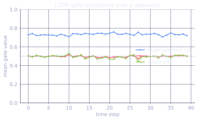
A practical detail: initialize the forget gate's bias $b_f$ to a positive value (typically $+1$ or $+2$). Sigmoid then starts near 1, the forget gate starts "mostly open", and gradients propagate through long sequences at the start of training. Without this trick, early in training the network forgets everything and never learns long dependencies.

When LSTMs win and lose

Won (2014-2018): language modeling, machine translation, speech recognition, time-series forecasting.

Lost to Transformers (2017+): the global context, parallel training, and superior scaling of attention beat LSTMs on every NLP benchmark.

Still useful: streaming inference, very long context with limited memory, control/RL applications, and any domain where sequence is inherently online.

Bi-LSTM and stacked LSTM

• Bi-LSTM: stack a forward-time LSTM and a backward-time LSTM; concatenate their hidden states at each position. The output at every position sees the whole sequence in both directions. Standard for encoders.
• Stacked LSTM: multiple LSTM layers on top of each other. Like stacked MLPs but for sequences.

The next lesson combines these encoder-decoder LSTM stacks with attention to handle longer dependencies.

Check it on arrays

import numpy as np

rng = np.random.default_rng(0)

def sigmoid(z): return 1 / (1 + np.exp(-z))

def lstm_step(x, h_prev, c_prev, Wf, Wi, Wo, Wc, bf, bi, bo, bc):
    z = np.concatenate([x, h_prev])
    f = sigmoid(Wf @ z + bf)
    i = sigmoid(Wi @ z + bi)
    o = sigmoid(Wo @ z + bo)
    c_tilde = np.tanh(Wc @ z + bc)
    c = f * c_prev + i * c_tilde
    h = o * np.tanh(c)
    return h, c

T, d_x, d_h = 30, 5, 16
X = rng.normal(size=(T, d_x))

# Initialize LSTM weights with bf positive (the trick)
def init(out_dim, in_dim): return rng.normal(scale=0.1, size=(out_dim, in_dim))
Wf = init(d_h, d_x + d_h); bf = np.ones(d_h) * 1.0          # forget bias = 1
Wi = init(d_h, d_x + d_h); bi = np.zeros(d_h)
Wo = init(d_h, d_x + d_h); bo = np.zeros(d_h)
Wc = init(d_h, d_x + d_h); bc = np.zeros(d_h)

h = np.zeros(d_h); c = np.zeros(d_h)
H = []; C = []
for t in range(T):
    h, c = lstm_step(X[t], h, c, Wf, Wi, Wo, Wc, bf, bi, bo, bc)
    H.append(h); C.append(c)
H = np.array(H); C = np.array(C)
print(f"hidden state norm at t=0, 10, 20, 29: "
      f"{[round(np.linalg.norm(H[t]), 3) for t in [0, 10, 20, 29]]}")
print(f"cell state norm at t=0, 10, 20, 29:   "
      f"{[round(np.linalg.norm(C[t]), 3) for t in [0, 10, 20, 29]]}")

# Forget-gate magnitude over time tells us how much memory is preserved
forget_norms = []
h_prev, c_prev = np.zeros(d_h), np.zeros(d_h)
for t in range(T):
    z = np.concatenate([X[t], h_prev])
    f_gate = sigmoid(Wf @ z + bf)
    forget_norms.append(f_gate.mean())
    h_prev, c_prev = lstm_step(X[t], h_prev, c_prev, Wf, Wi, Wo, Wc, bf, bi, bo, bc)
print(f"mean forget-gate value: {round(np.mean(forget_norms), 3)}  "
      f"(starts near sigmoid(1)=0.73)")

The cell state norm remains stable across 30 timesteps because the forget gate (initialized to bias +1) is mostly open.

Exercises

Exercise 1. One LSTM unit has previous cell state $c_{t-1} = 0.8$ and gate/candidate values $f_t = 0.9$, $i_t = 0.5$, $\tilde c_t = -0.4$, $o_t = 0.6$. Compute the new cell state $c_t$ and hidden state $h_t$ by hand. Use $\tanh(0.52) \approx 0.4777$.

Exercise 2. A memory unit must hold a value over $50$ steps. Compare the gradient decay of the LSTM cell path against a vanilla RNN whose recurrence Jacobian has spectral norm $0.9$. Assume the forget gate holds at $f_t = 0.98$ for all $50$ steps. Which path preserves the signal, and by what factor do they differ?

Exercise 3 (code). Implement one GRU step in numpy and verify the convex-combination property of its update: when the update gate $z_t = 1$ the new hidden state equals the candidate $\tilde h_t$, and when $z_t = 0$ it equals the previous state $h_{t-1}$, with intermediate $z_t$ interpolating between them.

import numpy as np

rng = np.random.default_rng(0)

def sigmoid(z): return 1 / (1 + np.exp(-z))

d_x, d_h = 4, 6

def gru_step(x, h_prev, Wz, Wr, Wh, bz, br, bh):
    z = sigmoid(Wz @ np.concatenate([x, h_prev]) + bz)
    r = sigmoid(Wr @ np.concatenate([x, h_prev]) + br)
    h_tilde = np.tanh(Wh @ np.concatenate([x, r * h_prev]) + bh)
    h = (1 - z) * h_prev + z * h_tilde
    return h, z, h_tilde

def init(o, i): return rng.normal(scale=0.5, size=(o, i))
Wz, Wr, Wh = init(d_h, d_x + d_h), init(d_h, d_x + d_h), init(d_h, d_x + d_h)
bz, br, bh = rng.normal(size=d_h), rng.normal(size=d_h), rng.normal(size=d_h)

x = rng.normal(size=d_x)
h_prev = rng.normal(size=d_h)
h, z, h_tilde = gru_step(x, h_prev, Wz, Wr, Wh, bz, br, bh)

# The update is a per-unit convex combination of h_prev and h_tilde
recombined = (1 - z) * h_prev + z * h_tilde
assert np.allclose(h, recombined)
# Forcing z = 0 keeps the old state; z = 1 takes the candidate
assert np.allclose((1 - 0) * h_prev + 0 * h_tilde, h_prev)
assert np.allclose((1 - 1) * h_prev + 1 * h_tilde, h_tilde)
# h lies between h_prev and h_tilde componentwise
lo = np.minimum(h_prev, h_tilde); hi = np.maximum(h_prev, h_tilde)
assert np.all((h >= lo - 1e-12) & (h <= hi + 1e-12))
print("z range:", round(z.min(), 3), "to", round(z.max(), 3))
print("h within [min, max] of (h_prev, h_tilde):", bool(np.all((h >= lo - 1e-12) & (h <= hi + 1e-12))))

The next lesson combines LSTMs with attention to handle variable-length input-output pairs.

References

- [1]Hochreiter, S., & Schmidhuber, J. (1997). "Long short-term memory". Neural Computation, 9(8), 1735-1780. doi:10.1162/neco.1997.9.8.1735. The original LSTM cell with forget, input, and output gates.↩
- [2]Cho, K., et al. (2014). "Learning phrase representations using RNN encoder-decoder (GRU)". EMNLP. arXiv:1406.1078. Introduces the gated recurrent unit.↩