t-SNE and UMAP

PCA finds the directions of largest variance, which is great for linear structure but terrible at preserving local neighborhoods on curved manifolds. t-SNE and UMAP are nonlinear, neighborhood-preserving methods designed specifically for visualization in 2D or 3D. They are indispensable for exploring embeddings and unsupervised structure, with characteristic failure modes you must know to read them right.

The shared idea

Both methods:

1. Build a graph of pairwise similarities in the high-dimensional space.
2. Initialize a low-dimensional embedding.
3. Iteratively move embedded points so the low-dimensional similarities match the high-dimensional ones, by gradient descent on a divergence.

The differences are in the similarity definition, the divergence, and the optimization.

t-SNE

In the high-dimensional space, t-SNE uses a Gaussian centered at each point; the perplexity parameter sets the effective neighborhood size (typically 5-50). Similarities are symmetrized into a joint distribution $P$.

In the low-dimensional space, similarities use a Student-t distribution (heavy-tailed) so that distant points have nonnegligible "repulsion":

Minimize KL divergence $D_{\text{KL}}(P \| Q)$ by gradient descent on the $y_i$. The heavy tail prevents the crowding problem: in low dimensions there is less room to spread points apart, and the t-distribution accommodates this[1].

UMAP

UMAP defines high-dimensional similarities using local connectivity: each point connects to its $k$ nearest neighbors with weights that decay with distance, calibrated so the local connectivity is constant across the manifold.

In the low-dimensional space, UMAP minimizes a binary cross-entropy between the connection probabilities under the high- and low-dimensional fuzzy simplicial set representations. The optimization uses stochastic gradient descent with explicit attraction (between connected points) and repulsion (between random non-edges).

UMAP is faster than t-SNE, better preserves global structure (because the optimization keeps non-neighbors apart, not just neighbors close), and supports out-of-sample transformation[2].

Hyperparameters that matter

t-SNE: perplexity. Controls the effective neighborhood size. Small perplexity emphasizes local structure; large perplexity blends in more global structure. Results are sensitive; sweeping a few values (5, 30, 50) is standard.

UMAP: n_neighbors. Similar role to perplexity. Default 15 works well.

UMAP: min_dist. How tightly points may cluster in the embedding. Smaller = tighter clusters, larger = more spread.

Pitfalls (read these before interpreting a t-SNE plot)

• Distances in the plot are not metric. The relative size of clusters, and the distance between clusters, in a t-SNE plot is not meaningful. Only neighborhood structure is preserved.
• Cluster shapes are not meaningful. The size and shape of each cluster is largely an artifact of perplexity and optimization, not the data.
• Hyperparameter sensitivity. Different perplexities can produce qualitatively different plots. Show several to avoid cherry-picking.
• Stochasticity. Different random seeds give different layouts. Run a few times to check stability.
• Not for downstream learning. Use the original high-dimensional representation, or learned embeddings, as input to a classifier. The t-SNE / UMAP output is a visualization aid, not a feature.

UMAP suffers from the same issues to a lesser degree because of its more principled global optimization, but the warnings apply to it too.

Check it on arrays

This is a minimalist t-SNE for the visualization pattern. Use scikit-learn or umap-learn in production.

import numpy as np

rng = np.random.default_rng(0)

# Three Gaussian blobs in 5D
n_per = 60
centers = [np.array([5, 0, 0, 0, 0]), np.array([-5, 0, 0, 0, 0]), np.array([0, 5, 0, 0, 0])]
X = np.vstack([rng.normal(loc=c, scale=1.0, size=(n_per, 5)) for c in centers])
y_true = np.array([0] * n_per + [1] * n_per + [2] * n_per)

def tsne_simple(X, n_components=2, perplexity=20, n_iter=500, lr=200, rng=rng):
    n, d = X.shape
    D2 = np.sum((X[:, None] - X[None, :])**2, axis=2)
    # Calibrate per-point sigma so the entropy ~ log(perplexity); use a single sigma here for simplicity
    sigma = np.std(X) * 2
    P_unnorm = np.exp(-D2 / (2 * sigma**2))
    np.fill_diagonal(P_unnorm, 0)
    P = P_unnorm / P_unnorm.sum()
    P = 0.5 * (P + P.T)
    Y = rng.normal(scale=1e-4, size=(n, n_components))
    for it in range(n_iter):
        d2_low = np.sum((Y[:, None] - Y[None, :])**2, axis=2)
        Q_unnorm = 1 / (1 + d2_low)
        np.fill_diagonal(Q_unnorm, 0)
        Q = Q_unnorm / Q_unnorm.sum()
        grad = np.zeros_like(Y)
        for i in range(n):
            diff = Y[i] - Y
            weights = 4 * (P[i] - Q[i]) * Q_unnorm[i]
            grad[i] = (weights[:, None] * diff).sum(axis=0)
        Y -= lr * grad
    return Y

Y = tsne_simple(X, perplexity=20, n_iter=300)
print(f"t-SNE embedding shape: {Y.shape}")
print("class-mean Y per cluster (should be separated):")
for c in range(3):
    print(f"  class {c}: mean Y = {Y[y_true == c].mean(axis=0).round(2)}")

# Compare to PCA: linear projection of the same data
from numpy.linalg import eigh
cov = np.cov(X.T)
vals, vecs = eigh(cov)
Y_pca = X @ vecs[:, ::-1][:, :2]
print("\nPCA embedding class-means:")
for c in range(3):
    print(f"  class {c}: mean Y = {Y_pca[y_true == c].mean(axis=0).round(2)}")
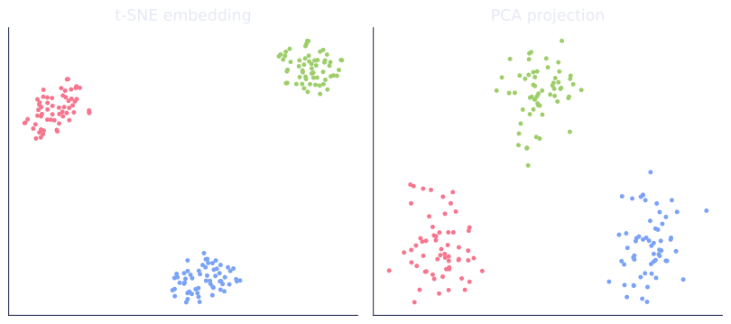
print("\nPCA does fine here because separation is linear; on curved manifolds, t-SNE/UMAP win.")

The t-SNE embedding pulls the three blobs apart in 2D, and PCA does the same on this linearly separable example.

Exercises

Exercise 1. In a t-SNE plot, two well-separated clusters appear with one twice the diameter of the other, and they sit far apart on the page. State which of these two visual facts (relative cluster size, between-cluster distance) you may report as a property of the data, and justify it from how t-SNE builds the embedding.

Exercise 2. The t-SNE low-dimensional kernel is $(1 + \lVert y_i - y_j \rVert^2)^{-1}$. Compare its tail to a Gaussian kernel $\exp(-\lVert y_i - y_j \rVert^2)$ at a large separation $r = \lVert y_i - y_j \rVert$, and explain how the heavier tail addresses the crowding problem.

Exercise 3 (code). On three well-separated 5D blobs, run the lesson's minimal t-SNE and verify the three class centroids in the 2D embedding are mutually farther apart than the within-class spread, the separation the plot is meant to show.

import numpy as np

rng = np.random.default_rng(0)
n_per = 60
centers = [np.array([6, 0, 0, 0, 0]), np.array([-6, 0, 0, 0, 0]), np.array([0, 6, 0, 0, 0])]
X = np.vstack([rng.normal(loc=c, scale=1.0, size=(n_per, 5)) for c in centers])
y = np.array([0] * n_per + [1] * n_per + [2] * n_per)

def tsne_simple(X, n_iter=300, lr=200, rng=rng):
    n = len(X)
    D2 = np.sum((X[:, None] - X[None, :])**2, axis=2)
    sigma = np.std(X) * 2
    P = np.exp(-D2 / (2 * sigma**2))
    np.fill_diagonal(P, 0)
    P = P / P.sum()
    P = 0.5 * (P + P.T)
    Y = rng.normal(scale=1e-4, size=(n, 2))
    for _ in range(n_iter):
        d2 = np.sum((Y[:, None] - Y[None, :])**2, axis=2)
        Qn = 1 / (1 + d2)
        np.fill_diagonal(Qn, 0)
        Q = Qn / Qn.sum()
        grad = np.zeros_like(Y)
        for i in range(n):
            w = 4 * (P[i] - Q[i]) * Qn[i]
            grad[i] = (w[:, None] * (Y[i] - Y)).sum(axis=0)
        Y -= lr * grad
    return Y

Y = tsne_simple(X)
cent = np.array([Y[y == c].mean(axis=0) for c in range(3)])
spread = np.mean([np.linalg.norm(Y[y == c] - cent[c], axis=1).mean() for c in range(3)])
min_between = min(np.linalg.norm(cent[a] - cent[b])
                  for a in range(3) for b in range(a + 1, 3))

assert min_between > spread                         # clusters separate cleanly
print("min between-centroid distance:", round(float(min_between), 2))
print("mean within-class spread:", round(float(spread), 2))

This closes C5 on unsupervised learning; the next subsection turns to detecting points that do not belong to any cluster: anomalies.

References

- [1]van der Maaten, L., & Hinton, G. (2008). "Visualizing data using t-SNE". JMLR, 9, 2579-2605. The Student-t low-dimensional kernel and the crowding problem.↩
- [2]McInnes, L., Healy, J., & Melville, J. (2018). "UMAP: uniform manifold approximation and projection for dimension reduction". arXiv:1802.03426. Fuzzy simplicial sets, the cross-entropy objective, and faster optimization.↩