k-medoids and robust centers

k-means uses cluster means as centers, which requires a meaningful mean. For non-Euclidean distances (cosine, Manhattan, Hamming, edit) or for data where outliers blow up means, k-medoids is the natural alternative: each cluster's center is an actual data point (a medoid) that minimizes the total distance to the others in its cluster[1].

The objective

Pick $k$ data points $m_1, \dots, m_k$ from the dataset as medoids, and minimize

where $d$ is any distance (or even a non-metric dissimilarity). Compared to k-means, the squared Euclidean is replaced by arbitrary $d$, and centers are constrained to be actual points.

PAM (Partition Around Medoids)

The classic algorithm[1]. After initialization:

1. Assignment: each point goes to its closest medoid.
2. Update: for each cluster, find the point that minimizes the total in-cluster distance and make it the new medoid. Equivalently, try swapping each non-medoid with each medoid and accept the swap if it lowers $J$.

PAM converges to a local minimum but is expensive: each update step is $O(k(n - k)^2)$ in the swap formulation. Modern variants (CLARA, CLARANS, FastPAM) trade exactness for speed.

Why use k-medoids

• Non-Euclidean distances: cosine, Manhattan, Hamming, Jaccard, edit distance. Any of these makes "the mean" undefined or meaningless, but k-medoids only needs to evaluate distances.
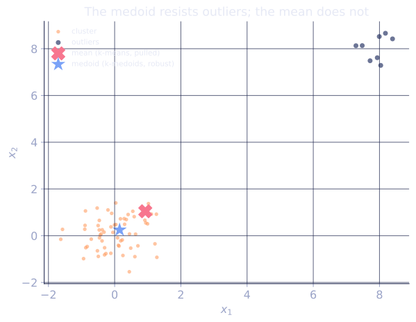
• Outlier robustness: a medoid minimizes total distance (an $L_1$-style criterion), so it sits near the bulk of the cluster, not pulled toward outliers the way a mean is.
• Interpretability: each center is an actual example, which is useful for explanation ("this cluster is best represented by document X").

Limits

• Slower than k-means by orders of magnitude: each iteration is superlinear in cluster size.
• Restricted to data points: cannot place a center between two clusters, which sometimes hurts inertia compared to k-means.

For large datasets, prefer PAM-like sampling methods (CLARANS), or use k-means on an embedded representation (apply PCA or learned embeddings, then cluster with k-means there)[2].

k-medians: the closely related cousin

Replacing the cluster center with the geometric median (the point minimizing total Euclidean distance, not mean) gives k-medians, which is robust to outliers but does not require centers to be data points. The geometric median has no closed form but is computed by Weiszfeld's algorithm.

Check it on arrays

import numpy as np

rng = np.random.default_rng(0)

# Two blobs + a handful of outliers
X = np.vstack([
    rng.normal(loc=[2.0, 0.0], scale=0.5, size=(80, 2)),
    rng.normal(loc=[-2.0, 0.0], scale=0.5, size=(80, 2)),
    np.array([[20.0, 20.0], [-20.0, -20.0]])         # extreme outliers
])
n = len(X)

def kmedoids(X, k, d, max_iter=100, init=None):
    n = len(X)
    if init is None:
        medoids = np.array(sorted(np.random.default_rng(0).choice(n, k, replace=False)))
    else:
        medoids = init
    D = d(X[:, None], X[None, :])                       # n x n distance matrix
    for _ in range(max_iter):
        # assign
        z = D[:, medoids].argmin(axis=1)
        # update each medoid as the point minimizing total distance within its cluster
        new_medoids = medoids.copy()
        for j in range(k):
            in_c = np.where(z == j)[0]
            if len(in_c) == 0: continue
            costs = D[np.ix_(in_c, in_c)].sum(axis=1)
            new_medoids[j] = in_c[np.argmin(costs)]
        if np.array_equal(np.sort(medoids), np.sort(new_medoids)):
            break
        medoids = new_medoids
    return medoids, z

# Use L1 (Manhattan) distance: no "mean" interpretation, but a clear medoid
def l1(a, b): return np.abs(a - b).sum(axis=-1)
medoids, z = kmedoids(X, 2, d=l1)
print(f"k-medoids with L1: medoid coordinates (actual data points):")
print(X[medoids].round(2))

# Compare to k-means with squared Euclidean (sensitive to outliers)
def kmeans_simple(X, k, max_iter=100, init=None):
    if init is None:
        mu = X[np.random.default_rng(0).choice(len(X), k, replace=False)]
    else:
        mu = X[init].copy()
    for _ in range(max_iter):
        d2 = ((X[:, None] - mu[None, :])**2).sum(axis=2)
        z = d2.argmin(axis=1)
        mu_new = np.array([X[z == j].mean(axis=0) if (z == j).sum() else mu[j] for j in range(k)])
        if np.allclose(mu, mu_new): break
        mu = mu_new
    return mu, z

mu_km, z_km = kmeans_simple(X, 2)
print(f"\nk-means centers (pulled toward outliers):")
print(mu_km.round(2))
print("\nk-medoids stays near the bulk; k-means centers shift toward the extreme points.")

The k-medoids centers are actual data points near each blob; k-means' centers are dragged toward the extreme outliers.

Exercises

Exercise 1. A one-dimensional cluster holds the points $\{1, 2, 3, 4, 100\}$. Find the medoid (the data point minimizing total absolute distance to the others) and the mean, and report how far each sits from the bulk $\{1, 2, 3, 4\}$.

Exercise 2. Explain why the k-medoids objective $J = \sum_i \min_j d(x_i, m_j)$ is well defined for a cosine dissimilarity while the k-means objective is not, and state the one structural constraint k-medoids adds compared to k-means.

Exercise 3 (code). With the L1 distance, compare a medoid (the in-cluster point of minimum total distance) against the coordinate-wise mean on a blob contaminated by one extreme outlier. Verify the medoid stays near the blob center while the mean is dragged far out.

import numpy as np

rng = np.random.default_rng(0)
blob = rng.normal(loc=[0.0, 0.0], scale=0.5, size=(50, 2))
X = np.vstack([blob, np.array([[50.0, 50.0]])])    # one extreme outlier

def l1(a, b):
    return np.abs(a - b).sum(axis=-1)

# medoid: data point minimizing total L1 distance to all others
D = l1(X[:, None], X[None, :])
medoid = X[D.sum(axis=1).argmin()]
mean = X.mean(axis=0)

# medoid stays inside the blob; mean is pulled toward the outlier
assert np.linalg.norm(medoid) < 2.0
assert np.linalg.norm(mean) > 0.8
print("medoid:", medoid.round(2), " dist from origin:", round(float(np.linalg.norm(medoid)), 2))
print("mean:  ", mean.round(2), " dist from origin:", round(float(np.linalg.norm(mean)), 2))

The next lesson takes a completely different geometric stance: clusters are dense regions, identified by DBSCAN.

References

- [1]Kaufman, L., & Rousseeuw, P. J. (1990). Finding Groups in Data: An Introduction to Cluster Analysis. Wiley. Introduces medoids and the PAM algorithm (Ch. 2).↩
- [2]Hastie, T., Tibshirani, R., & Friedman, J. (2009). The Elements of Statistical Learning (2nd ed.). Springer, §14.3.10. doi:10.1007/978-0-387-84858-7.↩