DBSCAN

k-means assumes clusters are spherical blobs and forces every point into some cluster. DBSCAN[1] drops both assumptions: it defines clusters as density-connected regions, picks up clusters of arbitrary shape, and flags low-density points as noise. It is the right tool when you do not know $k$ in advance and clusters might be curved or interlaced.

Density-based concepts

Three definitions, parameterized by a radius $\varepsilon$ and a minimum neighbor count minPts:

• Core point: has at least minPts other points within $\varepsilon$.
• Border point: has fewer than minPts neighbors but lies within $\varepsilon$ of some core point.
• Noise point: neither core nor border.

A core point is density-reachable from any other core point through a chain of overlapping $\varepsilon$-neighborhoods. A cluster is a maximal set of density-reachable points (core + border)[1].

The algorithm

1. Mark all points unvisited.
2. Pick an unvisited point $p$. If it is a core point, start a new cluster: add $p$ and recursively add every density-reachable point from $p$. Otherwise mark $p$ as noise (it may later be reassigned to a cluster as a border point).
3. Repeat until all points are visited.

The result is a set of clusters of arbitrary shape, plus a noise pile. The number of clusters is determined by the data, not specified up front.

Strengths

• Arbitrary cluster shapes: works on rings, half-moons, blobs, anything density-connected.
• No $k$ needed: the data decides.
• Noise tolerance: outliers are flagged, not crammed into clusters.
• Deterministic: same data and same $\varepsilon$/minPts give the same clusters (modulo border-point assignment order).

Picking the hyperparameters

minPts is usually set to $2d$ or $d + 1$ where $d$ is the dimension; it controls the minimum cluster size.

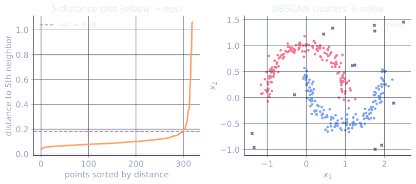
$\varepsilon$ is the harder one. Standard heuristic: plot the k-distance, the distance to each point's minPts-th nearest neighbor, sorted in ascending order. Look for a knee. Points to the left of the knee are core-eligible at the corresponding $\varepsilon$; points past the knee are noise-eligible.

The k-distance plot gives a defensible $\varepsilon$ choice without trial and error.

Limits

• Varying density: a single $\varepsilon$ either makes the dense clusters bleed together or misses the sparse ones. HDBSCAN (next lesson) fixes this.
• High dimensions: the curse of dimensionality (C4 lesson) makes density estimation unreliable[2].
• Border point ambiguity: a border point can be reached from multiple clusters; assignment depends on visit order. Usually a minor effect.

Check it on arrays

import numpy as np

rng = np.random.default_rng(0)

# Two interlocked half-moons + noise points
def make_moons(n_per=100, noise=0.1, rng=rng):
    t = np.linspace(0, np.pi, n_per)
    x1 = np.column_stack([np.cos(t), np.sin(t)])
    x2 = np.column_stack([1 - np.cos(t), 1 - np.sin(t) - 0.5])
    return np.vstack([x1, x2]) + noise * rng.normal(size=(2 * n_per, 2))

X_moons = make_moons(n_per=120)
X_noise = rng.uniform(-1.5, 2.5, size=(20, 2))
X = np.vstack([X_moons, X_noise])

def dbscan(X, eps, min_pts):
    n = len(X)
    labels = np.full(n, -1)                            # -1 = noise / unassigned
    visited = np.zeros(n, dtype=bool)
    D = np.linalg.norm(X[:, None] - X[None, :], axis=2)
    cluster_id = 0
    for i in range(n):
        if visited[i]: continue
        visited[i] = True
        neighbors = list(np.where(D[i] <= eps)[0])
        if len(neighbors) < min_pts:
            continue                                    # noise (provisionally)
        labels[i] = cluster_id
        seeds = list(neighbors)
        while seeds:
            j = seeds.pop()
            if not visited[j]:
                visited[j] = True
                nj = list(np.where(D[j] <= eps)[0])
                if len(nj) >= min_pts:
                    seeds.extend(nj)
            if labels[j] == -1:
                labels[j] = cluster_id
        cluster_id += 1
    return labels

labels = dbscan(X, eps=0.25, min_pts=5)
print(f"clusters found: {len(set(labels)) - (1 if -1 in labels else 0)}")
print(f"noise points: {(labels == -1).sum()} / {len(X)}")
for c in sorted(set(labels)):
    print(f"  label {c}: {int((labels == c).sum())} points")

# k-distance plot heuristic
k = 5
kdist = np.sort([np.partition(np.linalg.norm(X - x, axis=1), k)[k] for x in X])
print(f"\nk-distance percentiles for k={k}: 50%={np.percentile(kdist, 50):.3f}, 90%={np.percentile(kdist, 90):.3f}")
print("eps ~ knee of k-distance plot (around the percentile where the curve bends up)")

DBSCAN separates the two moons and labels the random points as noise; the k-distance plot suggests a reasonable $\varepsilon$.

Exercises

Exercise 1. Five points lie on a line at positions $0, 1, 2, 10, 11$. With $\varepsilon = 1.5$ and minPts $= 3$ (counting the point itself), classify each point as core, border, or noise.

Exercise 2. Explain why raising minPts while holding $\varepsilon$ fixed can only turn core points into non-core points (never the reverse), and what effect this has on the amount of data flagged as noise.

Exercise 3 (code). On one dense blob plus scattered uniform noise, run DBSCAN and verify it recovers a single cluster while flagging most of the scattered points as noise.

import numpy as np

rng = np.random.default_rng(0)
blob = rng.normal(loc=[0.0, 0.0], scale=0.3, size=(150, 2))
noise = rng.uniform(-5, 5, size=(30, 2))           # spread far from the blob
X = np.vstack([blob, noise])

def dbscan(X, eps, min_pts):
    n = len(X)
    labels = np.full(n, -1)
    visited = np.zeros(n, dtype=bool)
    D = np.linalg.norm(X[:, None] - X[None, :], axis=2)
    cid = 0
    for i in range(n):
        if visited[i]:
            continue
        visited[i] = True
        nb = list(np.where(D[i] <= eps)[0])
        if len(nb) < min_pts:
            continue
        labels[i] = cid
        seeds = list(nb)
        while seeds:
            j = seeds.pop()
            if not visited[j]:
                visited[j] = True
                nj = list(np.where(D[j] <= eps)[0])
                if len(nj) >= min_pts:
                    seeds.extend(nj)
            if labels[j] == -1:
                labels[j] = cid
        cid += 1
    return labels

labels = dbscan(X, eps=0.4, min_pts=5)
n_clusters = len(set(labels) - {-1})
n_noise = int((labels == -1).sum())

assert n_clusters == 1                              # the dense blob is one cluster
assert n_noise >= 20                                # most scattered points are noise
print("clusters:", n_clusters, " noise points:", n_noise)

The next lesson handles the varying-density case where one $\varepsilon$ is not enough: HDBSCAN.

References

- [1]Ester, M., Kriegel, H.-P., Sander, J., & Xu, X. (1996). "A density-based algorithm for discovering clusters in large spatial databases with noise". KDD. The original DBSCAN, core/border/noise points, and the k-distance heuristic for .↩
- [2]Hastie, T., Tibshirani, R., & Friedman, J. (2009). The Elements of Statistical Learning (2nd ed.). Springer. doi:10.1007/978-0-387-84858-7.↩