Hierarchical clustering

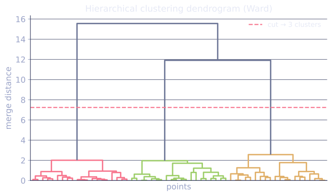
Hierarchical clustering builds a tree (dendrogram) instead of a flat partition: at the bottom, every point is its own cluster; at the top, one giant cluster[1]. The choice of linkage decides how distances between clusters are computed and produces very different dendrograms. Reading the dendrogram exposes structure at multiple scales.

Agglomerative vs divisive

• Agglomerative (bottom-up): start with $n$ singletons, repeatedly merge the two closest clusters until one remains.
• Divisive (top-down): start with one cluster, recursively split. Less common in practice (more expensive).

Agglomerative is the default. The merge order is recorded as a tree, and a flat clustering at any desired number of clusters is obtained by cutting the tree.

Four classical linkages

For clusters $A, B$ with pairwise distances $d(a, b)$:

• Single linkage: $d(A, B) = \min_{a \in A, b \in B} d(a, b)$. Produces "chained" elongated clusters, sensitive to noise bridges.
• Complete linkage: $d(A, B) = \max d(a, b)$. Produces compact, similarly-sized clusters; sensitive to outliers.
• Average linkage: $d(A, B) = \operatorname{avg}\, d(a, b)$. Compromise between single and complete.
• Ward's linkage: merges the two clusters whose union minimizes the increase in within-cluster sum of squares. Tends to produce balanced, spherical clusters; the natural choice for Euclidean data[2].

Different linkages can give entirely different clusterings on the same data. Picking one is a domain decision, not a default.

Reading the dendrogram

The y-axis of the dendrogram is the merge distance. A horizontal cut at height $h$ produces a flat clustering with one cluster per branch crossing the cut.

• Long vertical edges correspond to merges across a large distance jump: high stability at intermediate cuts.
• Many short merges near the bottom mean dense local structure.
• A clear "gap" of vertical space suggests a natural number of clusters (cut just below it).

Cost

Naive agglomerative clustering is $O(n^3)$ in time and $O(n^2)$ in memory because every pairwise distance is maintained. Approximate variants (BIRCH, mini-batch) bring this down for large $n$, but hierarchical clustering is the slowest classical clusterer.

When to use

• Need a hierarchy: phylogenies, taxonomies, document topic trees.
• Small $n$: a few hundred to a few thousand points fits easily.
• Don't know $k$: the dendrogram suggests good cut points visually.
• Non-Euclidean distances: works with any distance, like k-medoids but produces a tree.

Check it on arrays

import numpy as np

rng = np.random.default_rng(0)

# Three Gaussian blobs
X = np.vstack([
    rng.normal(loc=[2.0, 0.0], scale=0.4, size=(20, 2)),
    rng.normal(loc=[-2.0, 0.0], scale=0.4, size=(20, 2)),
    rng.normal(loc=[0.0, 2.0], scale=0.4, size=(20, 2)),
])

def agglomerative(X, linkage="single"):
    n = len(X)
    D = np.linalg.norm(X[:, None] - X[None, :], axis=2)
    clusters = [{i} for i in range(n)]
    merges = []                                        # (a, b, merge_distance, new_size)
    sizes = [1] * n
    active = list(range(n))
    while len(active) > 1:
        # find the closest pair among active clusters
        best = (None, None, float("inf"))
        for ai in active:
            for bi in active:
                if ai >= bi: continue
                d = D[ai, bi]
                if d < best[2]: best = (ai, bi, d)
        a, b, dist = best
        merges.append((a, b, dist, sizes[a] + sizes[b]))
        clusters[a] = clusters[a] | clusters[b]
        for c in active:
            if c == a or c == b: continue
            if linkage == "single":
                new_d = min(D[a, c], D[b, c])
            elif linkage == "complete":
                new_d = max(D[a, c], D[b, c])
            elif linkage == "average":
                new_d = (sizes[a] * D[a, c] + sizes[b] * D[b, c]) / (sizes[a] + sizes[b])
            elif linkage == "ward":
                new_d = ((sizes[a] + sizes[c]) * D[a, c]**2
                         + (sizes[b] + sizes[c]) * D[b, c]**2
                         - sizes[c] * dist**2) / (sizes[a] + sizes[b] + sizes[c])
                new_d = np.sqrt(max(new_d, 0))
            D[a, c] = D[c, a] = new_d
        sizes[a] = sizes[a] + sizes[b]
        active.remove(b)
    return merges

# Compare linkages
for link in ["single", "complete", "average", "ward"]:
    merges = agglomerative(X.copy(), linkage=link)
    # Distance of the last few merges (top of dendrogram)
    top = [m[2] for m in merges[-5:]]
    print(f"{link:>10} linkage, last 5 merge distances: {[round(d, 2) for d in top]}")

# Cut to produce 3 clusters with single linkage
merges = agglomerative(X.copy(), linkage="ward")
# Walk through merges, stop when 3 clusters remain
n = len(X)
parent = list(range(n))
def find(x):
    while parent[x] != x: parent[x] = parent[parent[x]]; x = parent[x]
    return x
for a, b, dist, _ in merges:
    if len(set(find(i) for i in range(n))) == 3: break
    parent[find(b)] = find(a)
labels = np.array([find(i) for i in range(n)])
_, labels = np.unique(labels, return_inverse=True)
print(f"\nWard cut to 3 clusters: cluster sizes = {[int((labels == c).sum()) for c in set(labels)]}")

Each linkage produces a different set of merge distances. Cutting Ward's dendrogram at 3 clusters recovers the three blobs.

Exercises

Exercise 1. Four points sit on a line at $0, 1, 5, 6$. Build the agglomerative dendrogram under single linkage by hand: list the merges in order with their merge distances.

Exercise 2. Show that single linkage and complete linkage give the same first merge on any dataset, then give a small example where their second merge differs.

Exercise 3 (code). Implement single-linkage agglomerative clustering and verify on the four-point set $\{0, 1, 5, 6\}$ that the final merge distance is $4$, matching Exercise 1.

import numpy as np

X = np.array([[0.0], [1.0], [5.0], [6.0]])

def single_linkage(X):
    n = len(X)
    D = np.linalg.norm(X[:, None] - X[None, :], axis=2)
    active = list(range(n))
    merges = []
    while len(active) > 1:
        best = (None, None, np.inf)
        for ai in active:
            for bi in active:
                if ai < bi and D[ai, bi] < best[2]:
                    best = (ai, bi, D[ai, bi])
        a, b, dist = best
        merges.append(dist)
        for c in active:
            if c not in (a, b):
                D[a, c] = D[c, a] = min(D[a, c], D[b, c])   # single linkage
        active.remove(b)
    return merges

merges = single_linkage(X)
assert np.isclose(merges[0], 1.0)
assert np.isclose(merges[-1], 4.0)                 # final merge distance
print("merge distances:", [round(m, 1) for m in merges])

The next lesson takes a fundamentally different stance again: clusters as Gaussians fit by EM.

References

- [1]Kaufman, L., & Rousseeuw, P. J. (1990). Finding Groups in Data: An Introduction to Cluster Analysis. Wiley. Agglomerative and divisive methods, the linkages, and reading dendrograms (Ch. 5-6).↩
- [2]Hastie, T., Tibshirani, R., & Friedman, J. (2009). The Elements of Statistical Learning (2nd ed.). Springer, §14.3.12. doi:10.1007/978-0-387-84858-7. Linkage comparison and Ward's criterion.↩