Gaussian mixture models and EM

A Gaussian mixture model (GMM) describes data as drawn from a weighted sum of Gaussians, each with its own mean and covariance. Fitting it directly by MLE is hard, but expectation-maximization (EM)[1] alternates two simple steps: probabilistic cluster assignment (E-step) and Gaussian re-estimation (M-step). The result is a soft, covariance-aware generalization of k-means[2].

The model

For $K$ components with parameters $\{\pi_k, \mu_k, \Sigma_k\}$, the GMM density is

with mixing weights $\pi_k \ge 0$, $\sum_k \pi_k = 1$. Equivalently, draw a component $z \in \{1, \dots, K\}$ from a categorical with probabilities $\pi$, then draw $x \mid z \sim \mathcal{N}(\mu_z, \Sigma_z)$.

The log-likelihood

has the log-of-sum that prevents a closed-form MLE. EM solves it by introducing latent assignment variables.

The EM algorithm

Initialize parameters. Iterate:

E-step. Compute the responsibility that component $k$ takes for example $i$ under the current parameters:

M-step. Update parameters with responsibility-weighted MLE:

where $N_k = \sum_i \gamma_{ik}$ is the effective number of points assigned to component $k$.

Each iteration is guaranteed to not decrease the log-likelihood (proof via Jensen's inequality applied to the latent-variable formulation)[1]. The algorithm converges to a local maximum.

GMM as soft k-means

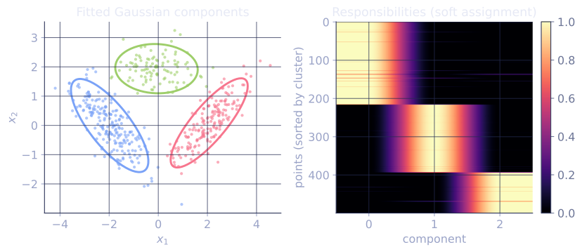
When $\Sigma_k = \sigma^2 I$ for all components and $\sigma \to 0$, responsibilities collapse to hard 0/1 assignments and the M-step reduces to mean update: GMM-EM becomes k-means. The general GMM relaxes k-means in two ways: covariance per cluster (elliptical, not spherical), and soft assignments (a point can belong fractionally to several clusters).

Initialization

EM is sensitive to local minima. The standard recipe:

1. Run k-means with multiple restarts to find good initial means.
2. Initialize each $\Sigma_k$ as the within-cluster covariance.
3. Initialize $\pi_k$ as the empirical cluster frequencies.

Then run EM to refine.

Choosing $K$

Use BIC or AIC:

with $p$ the number of free parameters ($K \cdot d + K \cdot d(d+1)/2 + (K - 1)$ for full covariances). Pick $K$ minimizing BIC. AIC uses $2p$ instead of $p\log n$ and tends to pick larger $K$.

For very large datasets and many components, variational Bayesian GMMs add a Dirichlet prior on $\pi$ that automatically prunes unnecessary components.

Strengths and limits

Strengths:

• Probabilistic model: gives data likelihood, component memberships, and density estimates.
• Captures elliptical clusters that k-means misses.
• Natural extension of k-means; same intuition.

Limits:

• Assumes Gaussian components. Curved or skewed clusters violate the assumption.
• Many parameters ($O(K d^2)$). For small samples per cluster, regularize covariances or restrict to diagonal.
• Component degeneracy: a component can collapse onto a single point, giving infinite likelihood. Regularize by adding $\varepsilon I$ to each $\Sigma_k$.

Check it on arrays

import numpy as np

rng = np.random.default_rng(0)

# Three elliptical clusters with different orientations
mu_true = [np.array([2.0, 0.0]), np.array([-2.0, 0.0]), np.array([0.0, 2.0])]
cov_true = [np.array([[1.0, 0.7], [0.7, 1.0]]),
            np.array([[1.0, -0.3], [-0.3, 0.3]]),
            np.array([[0.5, 0.0], [0.0, 0.5]])]
pi_true = np.array([0.4, 0.4, 0.2])
n = 500
z_true = rng.choice(3, size=n, p=pi_true)
# Draw z ~ N(0, I), then x = z @ L.T + mu  with  L L.T = Sigma  to get N(mu, Sigma).
X = np.vstack([rng.normal(size=(1, 2)) @ np.linalg.cholesky(cov_true[c]).T + mu_true[c]
               for c in z_true])

def log_gaussian(X, mu, Sigma):
    d = X.shape[1]
    diff = X - mu
    inv = np.linalg.inv(Sigma)
    sign, logdet = np.linalg.slogdet(Sigma)
    return -0.5 * d * np.log(2 * np.pi) - 0.5 * logdet - 0.5 * np.sum(diff @ inv * diff, axis=1)

def gmm_em(X, K, max_iter=100, tol=1e-5, rng=rng):
    n, d = X.shape
    # init: random points + identity covariance
    mu = X[rng.choice(n, K, replace=False)]
    Sigma = [np.eye(d) for _ in range(K)]
    pi = np.full(K, 1 / K)
    prev_ll = -np.inf
    for it in range(max_iter):
        # E-step
        log_resp = np.column_stack([log_gaussian(X, mu[k], Sigma[k]) + np.log(pi[k]) for k in range(K)])
        log_norm = np.logaddexp.reduce(log_resp, axis=1)
        log_resp -= log_norm[:, None]
        gamma = np.exp(log_resp)
        ll = log_norm.sum()
        if abs(ll - prev_ll) < tol: break
        prev_ll = ll
        # M-step
        Nk = gamma.sum(axis=0)
        pi = Nk / n
        for k in range(K):
            mu[k] = (gamma[:, k][:, None] * X).sum(axis=0) / Nk[k]
            diff = X - mu[k]
            Sigma[k] = (gamma[:, k][:, None] * diff).T @ diff / Nk[k] + 1e-4 * np.eye(d)
    return pi, mu, Sigma, gamma, ll

pi, mu, Sigma, gamma, ll = gmm_em(X, K=3)
print(f"log-likelihood: {ll:.2f}")
print(f"learned mixing weights: {pi.round(2)}, true: {pi_true.round(2)}")
print(f"learned means (sorted): \n{mu[np.argsort(mu[:, 0])].round(2)}")
print(f"true    means (sorted): \n{np.array(mu_true)[np.argsort([m[0] for m in mu_true])].round(2)}")

# BIC for K selection
def bic(X, K, pi, mu, Sigma, ll):
    n, d = X.shape
    p = K * d + K * d * (d + 1) // 2 + (K - 1)
    return -2 * ll + p * np.log(n)

for K in [1, 2, 3, 4, 5]:
    pi_k, mu_k, S_k, _, ll_k = gmm_em(X, K=K, rng=np.random.default_rng(K))
    print(f"K={K}: BIC = {bic(X, K, pi_k, mu_k, S_k, ll_k):.1f}")

GMM-EM recovers the mixing weights and means, the log-likelihood is monotonically increasing, and BIC correctly favors $K = 3$.

Exercises

Exercise 1. A two-component GMM has mixing weights $\pi = (0.6, 0.4)$. At a point $x$, the component densities are $\mathcal{N}(x \mid \mu_1, \Sigma_1) = 0.10$ and $\mathcal{N}(x \mid \mu_2, \Sigma_2) = 0.30$. Compute the responsibilities $\gamma_{x1}$ and $\gamma_{x2}$.

Exercise 2. Show that when $\Sigma_k = \sigma^2 I$ for all components with a common $\sigma$, the responsibilities reduce to a softmax over negative squared distances, and argue that as $\sigma \to 0$ this collapses to the hard k-means assignment.

Exercise 3 (code). Fit a two-component GMM with EM on data drawn from two Gaussians and verify that the per-iteration log-likelihood is non-decreasing, the monotonicity guaranteed by EM.

import numpy as np

rng = np.random.default_rng(0)
X = np.vstack([rng.normal(loc=[-3.0, 0.0], scale=1.0, size=(150, 2)),
               rng.normal(loc=[3.0, 0.0], scale=1.0, size=(150, 2))])

def log_gaussian(X, mu, Sigma):
    d = X.shape[1]
    diff = X - mu
    inv = np.linalg.inv(Sigma)
    _, logdet = np.linalg.slogdet(Sigma)
    return -0.5 * d * np.log(2 * np.pi) - 0.5 * logdet - 0.5 * np.sum(diff @ inv * diff, axis=1)

def gmm_em(X, K, max_iter=50, rng=rng):
    n, d = X.shape
    mu = X[rng.choice(n, K, replace=False)]
    Sigma = [np.eye(d) for _ in range(K)]
    pi = np.full(K, 1 / K)
    lls = []
    for _ in range(max_iter):
        log_resp = np.column_stack([log_gaussian(X, mu[k], Sigma[k]) + np.log(pi[k])
                                    for k in range(K)])
        log_norm = np.logaddexp.reduce(log_resp, axis=1)
        gamma = np.exp(log_resp - log_norm[:, None])
        lls.append(log_norm.sum())
        Nk = gamma.sum(axis=0)
        pi = Nk / n
        for k in range(K):
            mu[k] = (gamma[:, k][:, None] * X).sum(axis=0) / Nk[k]
            diff = X - mu[k]
            Sigma[k] = (gamma[:, k][:, None] * diff).T @ diff / Nk[k] + 1e-4 * np.eye(d)
    return np.array(lls)

lls = gmm_em(X, K=2)
# EM never decreases the log-likelihood from one iteration to the next
assert np.all(np.diff(lls) >= -1e-6)
print("first ll:", round(lls[0], 1), " last ll:", round(lls[-1], 1))

The final C5 lesson covers the visualization-focused dimensionality-reduction methods t-SNE and UMAP.

References

- [1]Dempster, A. P., Laird, N. M., & Rubin, D. B. (1977). "Maximum likelihood from incomplete data via the EM algorithm". JRSS-B, 39(1), 1-38. doi:10.1111/j.2517-6161.1977.tb01600.x. The general EM algorithm and its monotone-likelihood guarantee.↩
- [2]Hastie, T., Tibshirani, R., & Friedman, J. (2009). The Elements of Statistical Learning (2nd ed.). Springer, §8.5, §14.3. doi:10.1007/978-0-387-84858-7. GMMs, EM as soft k-means, and BIC/AIC model selection.↩