Linear and quadratic discriminant analysis

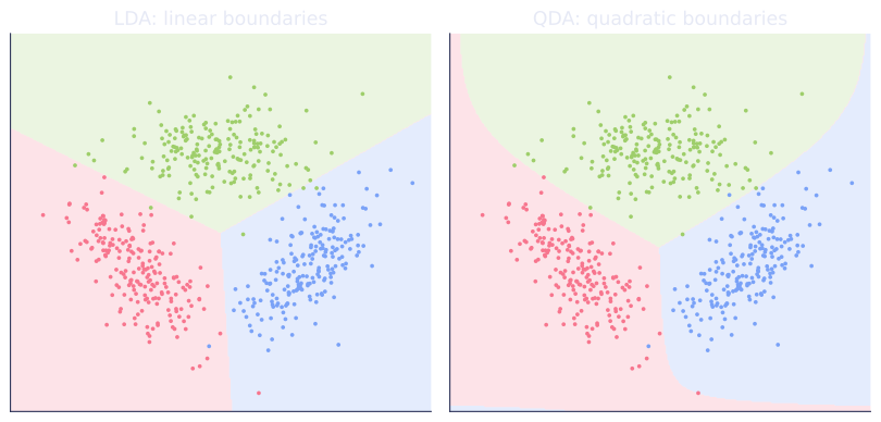
Naive Bayes assumes feature independence given the class. LDA and QDA drop that assumption: each class gets a full multivariate Gaussian, including covariances between features[1]. The shape of the decision boundary falls out of whether the classes share covariance or not.

The setup

Assume each class has a multivariate Gaussian class-conditional:

With class priors $\pi_c$, the Bayes-optimal classifier picks $\arg\max_c \pi_c\, \Pr(x \mid y = c)$. Taking the log, the discriminant function for class $c$ is

The classifier picks $\arg\max_c \delta_c(x)$.

QDA: per-class covariance

If each class has its own covariance $\Sigma_c$, the quadratic term in $\delta_c$ does not cancel across classes, so the decision boundary $\delta_a(x) = \delta_b(x)$ is quadratic in $x$. This is Quadratic Discriminant Analysis (QDA).

QDA has $O(d^2)$ parameters per class plus the prior, totaling roughly $C \cdot d^2$ parameters. With small training sets per class, the covariance estimates become unstable and the boundaries follow the noise.

LDA: shared covariance

If all classes share the same $\Sigma$, the quadratic term cancels in pairwise comparisons. The discriminant becomes

which is linear in $x$. The decision boundaries are hyperplanes; this is Linear Discriminant Analysis (LDA)[2].

LDA has only $O(C d + d^2)$ parameters and is more stable than QDA in small-sample regimes. It is the right starting point and what sklearn.discriminant_analysis.LinearDiscriminantAnalysis runs by default.

Regularized variants

When $\Sigma$ is ill-conditioned (small $n$, large $d$, or collinear features):

• Shrinkage LDA: $\Sigma \leftarrow (1 - \alpha)\hat\Sigma + \alpha\,\tfrac{\operatorname{tr}\hat\Sigma}{d}I$. Cross-validate $\alpha$. Especially useful in high-dimensional settings like text and genomics.
• Diagonal LDA: zero out off-diagonals of $\Sigma$. Equivalent to Gaussian Naive Bayes with shared variance per feature.

LDA vs logistic regression

Both produce linear decision boundaries. They differ in what they assume and optimize:

• LDA assumes Gaussian class-conditionals with shared covariance, fits by plug-in MLE on those Gaussians.
• Logistic regression assumes only that the log-odds are linear in $x$, fits by maximizing the conditional likelihood $\Pr(y \mid x)$[3].

When the LDA assumption is approximately correct, LDA tends to be more data-efficient. When it is grossly wrong (non-Gaussian features), logistic regression is more robust. Logistic also handles $y \mid x$ directly without needing to model $\Pr(x)$, which is appealing when $x$ is high-dimensional and unmodelable.

Check it on arrays

import numpy as np

rng = np.random.default_rng(0)

# Three classes with different covariances (QDA-favorable)
n_per = 200
mu = [np.array([2.0, 0.0]), np.array([-2.0, 0.0]), np.array([0.0, 2.0])]
cov = [np.array([[1.0, 0.0], [0.0, 0.5]]),
       np.array([[0.5, 0.0], [0.0, 1.0]]),
       np.array([[1.0, 0.7], [0.7, 1.0]])]

X, y = [], []
for c, (m, S) in enumerate(zip(mu, cov)):
    L = np.linalg.cholesky(S)
    Xc = rng.normal(size=(n_per, 2)) @ L.T + m
    X.append(Xc); y.extend([c] * n_per)
X = np.vstack(X); y = np.array(y)

idx = rng.permutation(len(y)); tr, te = idx[:400], idx[400:]
Xtr, ytr = X[tr], y[tr]; Xte, yte = X[te], y[te]

def fit_lda(X, y):
    classes = np.unique(y); d = X.shape[1]
    Sigma = np.zeros((d, d))
    means = {}; priors = {}
    for c in classes:
        Xc = X[y == c]
        mu_c = Xc.mean(axis=0)
        means[c] = mu_c; priors[c] = len(Xc) / len(X)
        Sigma += (Xc - mu_c).T @ (Xc - mu_c)
    Sigma /= len(X) - len(classes)
    return means, Sigma, priors

def fit_qda(X, y):
    classes = np.unique(y)
    params = {}
    for c in classes:
        Xc = X[y == c]
        mu_c = Xc.mean(axis=0); Sigma_c = np.cov(Xc.T) + 1e-4 * np.eye(Xc.shape[1])
        params[c] = (mu_c, Sigma_c, len(Xc) / len(X))
    return params

def predict_lda(X, means, Sigma, priors):
    inv = np.linalg.inv(Sigma); classes = list(means.keys())
    scores = []
    for c in classes:
        mu = means[c]
        s = X @ inv @ mu - 0.5 * mu @ inv @ mu + np.log(priors[c])
        scores.append(s)
    return np.array(classes)[np.argmax(scores, axis=0)]

def predict_qda(X, params):
    classes = list(params.keys()); scores = []
    for c, (mu, Sigma, pi) in params.items():
        inv = np.linalg.inv(Sigma)
        sign, logdet = np.linalg.slogdet(Sigma)
        diff = X - mu
        s = -0.5 * logdet - 0.5 * np.sum(diff @ inv * diff, axis=1) + np.log(pi)
        scores.append(s)
    return np.array(classes)[np.argmax(scores, axis=0)]

means, Sigma, priors = fit_lda(Xtr, ytr)
qda = fit_qda(Xtr, ytr)

print(f"LDA test acc: {np.mean(predict_lda(Xte, means, Sigma, priors) == yte):.3f}")
print(f"QDA test acc: {np.mean(predict_qda(Xte, qda) == yte):.3f}")
print("QDA wins when classes have different covariances; LDA wins when shared.")

QDA usually edges out LDA here because the three Gaussians have genuinely different covariances.

Exercises

Exercise 1. Take two classes with shared covariance $\Sigma = I$ (the $2\times 2$ identity), means $\mu_0 = (0, 0)$ and $\mu_1 = (2, 0)$, and equal priors $\pi_0 = \pi_1 = 1/2$. Using the LDA discriminant $\delta_c(x) = x^\top \Sigma^{-1}\mu_c - \tfrac12 \mu_c^\top \Sigma^{-1}\mu_c + \log\pi_c$, derive the decision boundary $\delta_0(x) = \delta_1(x)$ and state where it sits geometrically.

Exercise 2. QDA fits a separate covariance per class. Count the free parameters of QDA versus LDA for $C$ classes in $d$ dimensions (means, the covariance term, and $C - 1$ free priors). Evaluate both for $C = 10$, $d = 100$ and argue which is at greater risk of overfitting a small sample.

Exercise 3 (code). When the classes truly share a covariance, LDA should match or beat QDA, because QDA spends parameters estimating per-class covariances that are all the same. Generate three classes with a common covariance and a modest sample size, then compare LDA and QDA test accuracy, reusing the fitting code from the lesson.

import numpy as np

rng = np.random.default_rng(1)

# Shared covariance across all three classes (LDA-favorable), small sample.
n_per = 40
shared = np.array([[1.0, 0.6], [0.6, 1.0]])
L = np.linalg.cholesky(shared)
mu = [np.array([2.0, 0.0]), np.array([-2.0, 0.0]), np.array([0.0, 2.0])]
X, y = [], []
for c, m in enumerate(mu):
    X.append(rng.normal(size=(n_per, 2)) @ L.T + m)
    y.extend([c] * n_per)
X = np.vstack(X); y = np.array(y)

idx = rng.permutation(len(y)); tr, te = idx[:80], idx[80:]
Xtr, ytr = X[tr], y[tr]; Xte, yte = X[te], y[te]

def fit_lda(X, y):
    classes = np.unique(y); d = X.shape[1]
    Sigma = np.zeros((d, d)); means = {}; priors = {}
    for c in classes:
        Xc = X[y == c]; mu_c = Xc.mean(axis=0)
        means[c] = mu_c; priors[c] = len(Xc) / len(X)
        Sigma += (Xc - mu_c).T @ (Xc - mu_c)
    Sigma /= len(X) - len(classes)
    return means, Sigma, priors

def predict_lda(X, means, Sigma, priors):
    inv = np.linalg.inv(Sigma); classes = list(means.keys()); scores = []
    for c in classes:
        mu = means[c]
        scores.append(X @ inv @ mu - 0.5 * mu @ inv @ mu + np.log(priors[c]))
    return np.array(classes)[np.argmax(scores, axis=0)]

def fit_qda(X, y):
    classes = np.unique(y); params = {}
    for c in classes:
        Xc = X[y == c]
        params[c] = (Xc.mean(axis=0), np.cov(Xc.T) + 1e-4 * np.eye(Xc.shape[1]),
                     len(Xc) / len(X))
    return params

def predict_qda(X, params):
    classes = list(params.keys()); scores = []
    for c, (mu, Sigma, pi) in params.items():
        inv = np.linalg.inv(Sigma)
        _, logdet = np.linalg.slogdet(Sigma)
        diff = X - mu
        scores.append(-0.5 * logdet - 0.5 * np.sum(diff @ inv * diff, axis=1)
                      + np.log(pi))
    return np.array(classes)[np.argmax(scores, axis=0)]

means, Sigma, priors = fit_lda(Xtr, ytr)
qda = fit_qda(Xtr, ytr)
acc_lda = np.mean(predict_lda(Xte, means, Sigma, priors) == yte)
acc_qda = np.mean(predict_qda(Xte, qda) == yte)
print(f"LDA test acc: {acc_lda:.3f}")
print(f"QDA test acc: {acc_qda:.3f}")
assert acc_lda >= acc_qda

The next lesson reuses the LDA setup as a dimensionality-reduction method, the supervised twin of PCA.

References

- [1]Hastie, T., Tibshirani, R., & Friedman, J. (2009). The Elements of Statistical Learning (2nd ed.). Springer. LDA and QDA discriminants from Gaussian class-conditionals (§4.3) (doi:10.1007/978-0-387-84858-7).↩
- [2]Fisher, R. A. (1936). "The use of multiple measurements in taxonomic problems". Annals of Eugenics, 7(2), 179-188. The origin of linear discriminant analysis (doi:10.1111/j.1469-1809.1936.tb02137.x).↩
- [3]Bishop, C. M. (2006). Pattern Recognition and Machine Learning. Springer. Generative vs discriminative linear classifiers, LDA against logistic regression (§4.2-4.3).↩