k-nearest neighbors

The simplest learning rule: to predict for a new point, find the $k$ closest training examples and reuse their labels. k-nearest neighbors (k-NN) has no training step (it stores the data) and almost no inductive bias beyond "nearby points have similar labels"[1]. It is a useful baseline, a sanity check, and a stepping stone to the curse-of-dimensionality lesson that follows.

The algorithm

To predict for a query $x_\star$:

1. Compute distances $d(x_\star, x_i)$ to every training point.
2. Pick the $k$ nearest neighbors.
3. For classification: predict the majority class among the neighbors. For regression: predict their mean (or median for robustness).

There is no model to fit. Inference walks the entire training set, costing $O(n d)$ per query (which is what the C8 lessons on approximate nearest neighbor address).

Choosing $k$

$k$ is the regularization knob:

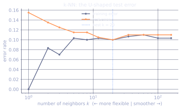
• $k = 1$: zero training error but enormous variance. Each prediction is determined by a single point, so noise dominates.
• $k$ large: low variance (averaging stabilizes the prediction) but high bias (averaging across distant points blurs the structure). $k = n$ predicts the global mean / majority everywhere.

Pick $k$ by cross-validation[2]. Common practice for classification: odd $k$ to avoid ties; values in the range $\sqrt{n}$ to $n/10$ are typical starting points.

Distance choices

• Euclidean ($L_2$): default for continuous features, after scaling.
• Manhattan ($L_1$): more robust to outliers.
• Cosine: for high-dimensional sparse representations (text, embeddings).
• Hamming: for binary or categorical features.

Whatever metric, features must be scaled before computing distances. A feature in dollars and one in millimeters will let the dollar feature dominate every distance computation if both are raw.

Weighted k-NN

Instead of all $k$ neighbors voting equally, weight each by $1/d$ or by a kernel of distance. Closer neighbors get more say. Smooths the predictor and makes $k$ less sensitive.

What k-NN does badly

• High dimensions: distances concentrate (next lesson), so every point is about as far as every other and the "nearest" neighbor barely means anything.
• Slow inference: $O(nd)$ per query; production systems use KD-trees, ball trees, or ANN indices (C8).
• Memory hungry: the model is the training set.
• No probabilities by default: vote fractions are uncalibrated.

Strengths

• Trivial to implement and reason about.
• No assumptions on the target's shape, smoothness, or distribution.
• Locally adapts: complex decision boundaries cost no extra fitting effort.
• Good baseline for tabular problems on small to medium $n$.

Check it on arrays

import numpy as np

rng = np.random.default_rng(0)

# Binary classification: two Gaussian blobs
n_per = 150
X_pos = rng.normal(loc=[1.5, 0.5], scale=0.7, size=(n_per, 2))
X_neg = rng.normal(loc=[-1.0, -0.5], scale=0.7, size=(n_per, 2))
X = np.vstack([X_pos, X_neg])
y = np.array([1] * n_per + [0] * n_per)

idx = rng.permutation(len(y))
tr, te = idx[:200], idx[200:]
Xtr, ytr = X[tr], y[tr]
Xte, yte = X[te], y[te]

def knn_predict(Xq, Xtr, ytr, k=5):
    d = np.sqrt(((Xq[:, None, :] - Xtr[None, :, :])**2).sum(axis=2))
    nn = np.argsort(d, axis=1)[:, :k]                  # k nearest indices per query
    votes = ytr[nn]
    # Majority vote (binary)
    return (votes.sum(axis=1) > k / 2).astype(int)

for k in [1, 3, 5, 11, 51]:
    y_pred = knn_predict(Xte, Xtr, ytr, k=k)
    acc = np.mean(y_pred == yte)
    print(f"k={k:>3}: test accuracy={acc:.3f}")

# Distance matters: add a noisy feature with a huge scale and watch the
# informative features get drowned out (no train/query mismatch, just
# a feature whose magnitude dominates the L2 distance).
noise_tr = 100.0 * rng.normal(size=(len(Xtr), 1))
noise_te = 100.0 * rng.normal(size=(len(Xte), 1))
Xtr_noisy = np.column_stack([Xtr, noise_tr])
Xte_noisy = np.column_stack([Xte, noise_te])
acc_bad = np.mean(knn_predict(Xte_noisy, Xtr_noisy, ytr, k=5) == yte)
acc_ok  = np.mean(knn_predict(Xte, Xtr, ytr, k=5) == yte)
print(f"\nwith a noisy feature on scale 100: acc={acc_bad:.3f}  (drowns out signal)")
print(f"informative features only:         acc={acc_ok:.3f}")

# Regression k-NN: average instead of vote
y_reg = X[:, 0] + 0.3 * rng.normal(size=len(X))
def knn_regress(Xq, Xtr, y_reg_tr, k=5):
    d = np.sqrt(((Xq[:, None, :] - Xtr[None, :, :])**2).sum(axis=2))
    nn = np.argsort(d, axis=1)[:, :k]
    return y_reg_tr[nn].mean(axis=1)

y_reg_tr = y_reg[tr]; y_reg_te = y_reg[te]
rmse = np.sqrt(np.mean((knn_regress(Xte, Xtr, y_reg_tr, k=10) - y_reg_te)**2))
print(f"k-NN regression test RMSE: {rmse:.3f}")

The U-shape in $k$ is visible: $k = 1$ overfits, large $k$ underfits, with the sweet spot in between. Adding one high-magnitude noise feature drowns out the informative ones, confirming the scaling caveat.

Exercises

Exercise 1. A 1-NN classifier is trained on the four labeled points $(0, +)$, $(1, +)$, $(3, -)$, $(5, -)$ on the real line, with distance $d(a, b) = |a - b|$. Predict the label at the query $x_\star = 2$ and at $x_\star = 2.5$, and find the location of the decision boundary between the $+$ and $-$ regions.

Exercise 2. With $k = n$ (every neighbor votes), show that k-NN classification predicts the global majority class at every query, and k-NN regression predicts the global mean of the training targets at every query. Explain why this is the maximum-bias, zero-variance end of the knob.

Exercise 3 (code). Implement distance-weighted k-NN classification, where each of the $k$ neighbors votes with weight $1/(d + \varepsilon)$ for a small $\varepsilon$ instead of weight $1$. On a two-blob problem, confirm that at $k = 15$ the weighted variant matches or beats uniform voting on test accuracy.

import numpy as np

rng = np.random.default_rng(0)

n_per = 150
X_pos = rng.normal(loc=[1.5, 0.5], scale=0.7, size=(n_per, 2))
X_neg = rng.normal(loc=[-1.0, -0.5], scale=0.7, size=(n_per, 2))
X = np.vstack([X_pos, X_neg])
y = np.array([1] * n_per + [0] * n_per)

idx = rng.permutation(len(y))
tr, te = idx[:200], idx[200:]
Xtr, ytr = X[tr], y[tr]
Xte, yte = X[te], y[te]

def dists(Xq, Xtr):
    return np.sqrt(((Xq[:, None, :] - Xtr[None, :, :]) ** 2).sum(axis=2))

def knn_uniform(Xq, Xtr, ytr, k):
    nn = np.argsort(dists(Xq, Xtr), axis=1)[:, :k]
    return (ytr[nn].sum(axis=1) > k / 2).astype(int)

def knn_weighted(Xq, Xtr, ytr, k, eps=1e-6):
    d = dists(Xq, Xtr)
    nn = np.argsort(d, axis=1)[:, :k]
    rows = np.arange(len(Xq))[:, None]
    w = 1.0 / (d[rows, nn] + eps)                  # weight per neighbor
    labels = ytr[nn]
    vote_pos = (w * (labels == 1)).sum(axis=1)
    vote_neg = (w * (labels == 0)).sum(axis=1)
    return (vote_pos > vote_neg).astype(int)

k = 15
acc_uniform = np.mean(knn_uniform(Xte, Xtr, ytr, k) == yte)
acc_weighted = np.mean(knn_weighted(Xte, Xtr, ytr, k) == yte)
print(f"uniform  k={k}: acc={acc_uniform:.3f}")
print(f"weighted k={k}: acc={acc_weighted:.3f}")
assert acc_weighted >= acc_uniform

The next lesson explains why all of this gets worse as the dimension grows.

References

- [1]Cover, T. M., & Hart, P. E. (1967). "Nearest neighbor pattern classification". IEEE Transactions on Information Theory, 13(1), 21-27. The original analysis of the nearest-neighbor rule and its asymptotic error bound (doi:10.1109/TIT.1967.1053964).↩
- [2]Hastie, T., Tibshirani, R., & Friedman, J. (2009). The Elements of Statistical Learning (2nd ed.). Springer. k-NN as a baseline and the bias-variance role of (§13.3) (doi:10.1007/978-0-387-84858-7).↩