Naive Bayes

Naive Bayes is the classifier you build when you accept a brutally simplifying assumption: features are conditionally independent given the class. The assumption is rarely true, but the resulting classifier is fast, needs little data, and works surprisingly well, especially as a baseline for text and other high-dimensional sparse problems[1].

The model

By Bayes' rule, the class posterior is

with $\pi_c = \Pr(y = c)$ the class prior. The full class-conditional $\Pr(x \mid y = c)$ is a joint distribution over all features, which is expensive to estimate when $d$ is large.

The naive assumption: features are independent given the class,

Now only $d$ one-dimensional distributions need to be fit per class. The classifier reduces to

Three concrete flavors

The feature type fixes the class-conditional family.

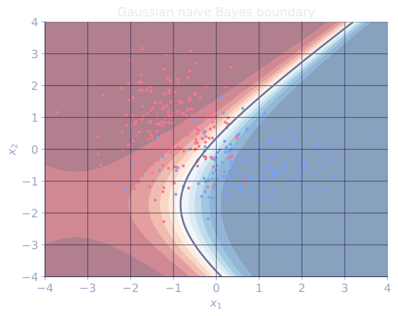
• Gaussian NB: continuous features, $\Pr(x_j \mid y = c) = \mathcal{N}(\mu_{cj}, \sigma_{cj}^2)$. Per-feature, per-class mean and variance estimated from data.
• Multinomial NB: count features (word counts in text), each class has a multinomial over the vocabulary. The score for a document becomes $\log \pi_c + \sum_j n_{xj}\log p_{cj}$ where $p_{cj}$ is the smoothed probability of word $j$ under class $c$.
• Bernoulli NB: binary features (word present / absent). Cheap and effective for short text.

Laplace (additive) smoothing

For count features, the MLE assigns probability zero to any word never seen in a class, which makes any document containing that word impossible under that class. The standard fix: add $\alpha > 0$ to every count,

with $V$ the vocabulary size. $\alpha = 1$ (Laplace smoothing) is standard. This is MAP under a symmetric Dirichlet prior[2].

Why it works despite the wrong assumption

Conditional independence is rarely true (especially for text), so the posterior probabilities Naive Bayes produces are usually badly calibrated. But the argmax is often correct: even badly calibrated probabilities can rank classes correctly. NB is therefore a strong classifier and a weak probability estimator[3].

The split between these two is the confusion worth pinning down, because the posterior and the decision can diverge sharply. Take a spam filter where two features fire together, the words "free" and "gratis", which co-occur almost perfectly. With equal priors and each feature carrying a likelihood ratio $\Pr(x_j \mid \text{spam}) / \Pr(x_j \mid \text{ham}) = 4$, NB multiplies them as if independent, combined ratio $4 \times 4 = 16$, giving posterior $16 / 17 \approx 0.94$. The honest answer treats the duplicated word as one piece of evidence, ratio $4$, posterior $4 / 5 = 0.8$. The probability is inflated by double-counting, but both clear $0.5$, so the argmax is spam either way. The decision survives the modeling error the calibrated probability does not.

When calibration matters (decisions weighted by probability), recalibrate with Platt scaling or isotonic regression (the calibration lesson in C9).

Strengths and limits

Strengths:

• Trivial to train: one pass over the data computes all per-feature, per- class statistics.
• Handles many features well, including text vocabularies.
• Strong baseline for text classification, spam filtering, and document categorization.
• Robust to irrelevant features (their per-class likelihoods cancel out).

Limits:

• Probabilities are usually badly miscalibrated.
• Strongly correlated features (which are common in text) compound: their evidence is double-counted.
• Continuous-feature Gaussian NB assumes per-class normality, which is rarely true.

Check it on arrays

import numpy as np

rng = np.random.default_rng(0)

# Gaussian NB on a 2-class, d-feature problem
n_per, d = 200, 4
mu_pos = np.array([1.0, -0.5, 0.5, 0.0])
mu_neg = np.array([-1.0, 0.5, -0.5, 0.0])
X_pos = rng.normal(loc=mu_pos, scale=1.0, size=(n_per, d))
X_neg = rng.normal(loc=mu_neg, scale=1.0, size=(n_per, d))
X = np.vstack([X_pos, X_neg]); y = np.array([1] * n_per + [0] * n_per)

idx = rng.permutation(len(y)); tr, te = idx[:300], idx[300:]
Xtr, ytr = X[tr], y[tr]; Xte, yte = X[te], y[te]

def fit_gaussian_nb(X, y):
    classes = np.unique(y)
    params = {}
    for c in classes:
        Xc = X[y == c]
        params[c] = (Xc.mean(axis=0), Xc.var(axis=0) + 1e-6, np.mean(y == c))
    return params

def predict_gaussian_nb(X, params):
    scores = []
    for c, (mu, var, pi) in params.items():
        log_lik = -0.5 * np.sum(np.log(2 * np.pi * var) + (X - mu)**2 / var, axis=1)
        scores.append(log_lik + np.log(pi))
    return np.array(list(params.keys()))[np.argmax(scores, axis=0)]

params = fit_gaussian_nb(Xtr, ytr)
print(f"Gaussian NB test acc: {np.mean(predict_gaussian_nb(Xte, params) == yte):.3f}")

# Multinomial NB on word-count features
vocab = 50; n_docs = 200
true_dist = [
    np.array([0.4] + [0.6 / (vocab - 1)] * (vocab - 1)),       # class 0: word 0 frequent
    np.concatenate([[0.6 / (vocab - 1)] * 30, [0.4], [0.6 / (vocab - 1)] * (vocab - 31)]),  # class 1: word 30 frequent
]
true_dist = [d / d.sum() for d in true_dist]
y_doc = rng.integers(0, 2, size=n_docs)
X_count = np.zeros((n_docs, vocab), dtype=int)
for i, c in enumerate(y_doc):
    X_count[i] = rng.multinomial(40, true_dist[c])

def fit_multinomial_nb(X, y, alpha=1.0):
    classes = np.unique(y); V = X.shape[1]
    p = {}
    for c in classes:
        counts = X[y == c].sum(axis=0)
        p[c] = ((counts + alpha) / (counts.sum() + alpha * V), np.mean(y == c))
    return p

def predict_multinomial_nb(X, p):
    classes = np.array(list(p.keys()))
    log_probs = np.stack([np.log(p[c][1]) + X @ np.log(p[c][0]) for c in classes], axis=0)
    return classes[np.argmax(log_probs, axis=0)]

idx = rng.permutation(n_docs); tr, te = idx[:150], idx[150:]
mnb = fit_multinomial_nb(X_count[tr], y_doc[tr])
print(f"Multinomial NB test acc: {np.mean(predict_multinomial_nb(X_count[te], mnb) == y_doc[te]):.3f}")

Both NB flavors classify their respective tasks well.

Exercises

Exercise 1. A Bernoulli Naive Bayes spam filter uses two binary word features. The class priors are equal, $\pi_{\text{spam}} = \pi_{\text{ham}} = 0.5$. For the word "win," $\Pr(\text{win} \mid \text{spam}) = 0.6$ and $\Pr(\text{win} \mid \text{ham}) = 0.1$. For the word "meeting," $\Pr(\text{meeting} \mid \text{spam}) = 0.1$ and $\Pr(\text{meeting} \mid \text{ham}) = 0.5$. A message contains "win" and not "meeting." Compute the posterior $\Pr(\text{spam} \mid x)$ by hand under the naive assumption.

Exercise 2. A class has seen a vocabulary word $j$ exactly $n_{cj} = 0$ times, with the class's total count $\sum_k n_{ck} = 100$ and vocabulary size $V = 1000$. Compute the smoothed probability $p_{cj}$ under Laplace smoothing ($\alpha = 1$), and explain in one sentence what the unsmoothed MLE would do to the score of any document containing word $j$.

Exercise 3 (code). The lesson claims correlated features inflate Naive Bayes posteriors by double-counting evidence. Build a 2-feature Gaussian NB problem where the two features are duplicates (perfectly correlated within each class). Show that the NB posterior at a test point is more extreme (closer to $0$ or $1$) than the posterior from a single copy of the feature, while the argmax label is unchanged.

import numpy as np

rng = np.random.default_rng(0)

# One informative feature: class means +1 / -1, unit variance, equal priors.
mu = {1: 1.0, 0: -1.0}
var = 1.0

def log_post_spam(x_vec, means):
    # Gaussian NB log-scores for a single test vector over given feature means.
    scores = {}
    for c in (0, 1):
        ll = -0.5 * np.sum(np.log(2 * np.pi * var) + (x_vec - means[c]) ** 2 / var)
        scores[c] = ll + np.log(0.5)              # equal priors
    m = max(scores.values())
    p1 = np.exp(scores[1] - m)
    p0 = np.exp(scores[0] - m)
    return p1 / (p1 + p0), int(scores[1] > scores[0])

x = 0.5                                            # test point on the + side

# Single feature
post1, lab1 = log_post_spam(np.array([x]), {1: np.array([mu[1]]), 0: np.array([mu[0]])})

# Duplicated feature: NB treats the two identical copies as independent
post2, lab2 = log_post_spam(np.array([x, x]),
                            {1: np.array([mu[1], mu[1]]), 0: np.array([mu[0], mu[0]])})

print(f"single-feature posterior P(y=1): {post1:.4f}, label {lab1}")
print(f"duplicated-feature posterior   : {post2:.4f}, label {lab2}")
assert post2 > post1            # double-counting pushes the posterior more extreme
assert lab1 == lab2             # but the decision is unchanged

The next lesson tightens the Gaussian-NB assumption to use full per-class covariance matrices: LDA and QDA.

References

- [1]Murphy, K. P. (2012). Machine Learning: A Probabilistic Perspective. MIT Press. Naive Bayes classifiers and their flavors (§3.5).↩
- [2]Bishop, C. M. (2006). Pattern Recognition and Machine Learning. Springer. Conjugate Dirichlet priors and MAP estimation for multinomial counts (§2.2).↩
- [3]Hastie, T., Tibshirani, R., & Friedman, J. (2009). The Elements of Statistical Learning (2nd ed.). Springer. Why Naive Bayes classifies well despite poor probability estimates (§6.6.3) (doi:10.1007/978-0-387-84858-7).↩