Distance metrics and the curse of dimensionality

In high dimensions, geometry stops behaving like the 2D picture in our heads. Distances concentrate: every pair of random points is about as far apart as every other. Nearest-neighbor methods lose their meaning. This curse of dimensionality[1] is not a flaw in any specific algorithm; it is a property of Euclidean space that constrains all distance-based methods.

Distance concentration

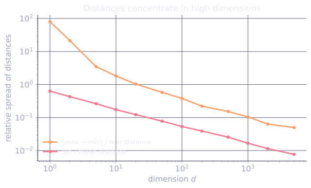
Sample $n$ points uniformly in the unit cube $[0, 1]^d$. As $d$ grows:

• All pairwise distances cluster around the same value.
• The ratio (max distance)/(min distance) approaches 1.

The empirical effect: in 1D the nearest neighbor of a query point is much closer than the farthest. In $d = 1000$, the nearest neighbor and the farthest are essentially the same distance away. "Nearest neighbor" stops being a meaningful concept.

Why. For a random unit-cube point, the squared distance to another random unit-cube point is $\sum_{j=1}^d (X_j - Y_j)^2$, a sum of $d$ i.i.d. random variables. By the central limit theorem the sum concentrates around its mean $d/6$ with standard deviation $\propto \sqrt d$. The relative spread $\sqrt d / d = 1/\sqrt d$ vanishes as $d \to \infty$. All distances look the same, relatively[2].

Volume in high dimensions

Two related facts that make the unit cube weird:

• Volume concentrates at the boundary. In $[0, 1]^d$ the fraction of volume within distance $0.1$ of any face is $1 - 0.9^d$. For $d = 50$ that is $99.5\%$. Most "interior" points are not interior.
• Volume escapes the inscribed ball. The volume of the unit ball inscribed in $[0, 1]^d$ goes to zero as $d \to \infty$, while the cube has volume 1. The ball occupies a vanishing fraction of the cube.

For k-NN, the practical effect: any reasonable distance threshold either captures almost everything or almost nothing as $d$ grows.

What survives, and why

• Low intrinsic dimension. If data live on a low-dimensional manifold embedded in high-dimensional space, distances in the ambient space can still be uninformative, but distances along the manifold are not. Methods like t-SNE and UMAP work because real data often have low intrinsic dimension even when raw features are high-dimensional.
• Sparse representations. In high-dimensional sparse vectors (text bag of words, one-hot categoricals), $L_1$ distance and cosine similarity often work better than Euclidean. Cosine ignores magnitude and focuses on the angle, which is robust to sparsity.
• Learned metrics. Metric learning and embedding models train a low- dimensional space where Euclidean distance is meaningful for the task at hand; that is what produces the "embeddings" used in vector databases (C8).

Practical guide for k-NN in high dimensions

• Reduce dimension first (PCA, autoencoders, learned embeddings) and apply k-NN in the reduced space.
• Use cosine for high-dimensional sparse vectors.
• Set $k$ larger to compensate for noisy distances.
• Be skeptical of small differences in distance; consider weighted voting rather than hard top-$k$.

The most defensible move is usually "don't use raw high-dimensional distances at all": embed first, then measure distances in the embedding.

Check it on arrays

import numpy as np

rng = np.random.default_rng(0)

# Pairwise distance ratio across increasing dimensions.
# Compute via ||x - y||^2 = ||x||^2 + ||y||^2 - 2 x^T y to avoid materializing
# the n x n x d broadcast (which would OOM at large d).
print(f"{'d':>5}  {'min':>8}  {'max':>8}  {'max/min':>8}  {'std/mean':>8}")
for d in [1, 2, 10, 100, 1000, 5000]:
    X = rng.random(size=(200, d))
    sq = (X * X).sum(axis=1)
    d2 = sq[:, None] + sq[None, :] - 2 * X @ X.T
    d2 = np.maximum(d2, 0.0)                          # clip tiny negatives
    d2_off = d2[~np.eye(len(X), dtype=bool)]
    dist = np.sqrt(d2_off)
    print(f"{d:>5}  {dist.min():>8.3f}  {dist.max():>8.3f}  "
          f"{dist.max() / dist.min():>8.3f}  {dist.std() / dist.mean():>8.3f}")

# Volume concentration at the boundary of the unit cube
d_grid = [2, 10, 50, 100]
for d in d_grid:
    # fraction within 0.05 of any face
    X = rng.random(size=(50000, d))
    inside = np.all((X > 0.05) & (X < 0.95), axis=1)
    print(f"d={d:>4}: fraction strictly inside (>0.05 from each face) = {inside.mean():.4f}")

As $d$ grows, the ratio of farthest to nearest pairwise distance approaches 1 and the relative spread of distances shrinks. In 100 dimensions, less than a half-percent of unit-cube points are even slightly away from the boundary.

Exercises

Exercise 1. For two points drawn uniformly from $[0, 1]^d$, the squared distance is $D^2 = \sum_{j=1}^d (X_j - Y_j)^2$ with the $(X_j - Y_j)^2$ terms i.i.d. A single coordinate gap $U = X_j - Y_j$ has $\mathbb{E}[U^2] = 1/6$. Use this to derive $\mathbb{E}[D^2] = d/6$, and explain why the relative spread $\operatorname{sd}(D^2)/\mathbb{E}[D^2]$ shrinks like $1/\sqrt d$.

Exercise 2. A query point sits at the center of $[0, 1]^d$. To capture a fraction $r$ of the unit-cube volume inside an axis-aligned subcube centered on the query, the subcube must have side length $s = r^{1/d}$. Compute $s$ for $r = 0.01$ at $d = 1$, $d = 10$, and $d = 100$, and state what this says about the size of a "local" neighborhood in high dimensions.

Exercise 3 (code). Distances concentrate, but a low intrinsic dimension rescues them. Generate data that lives on a 2D plane embedded in $d = 200$ ambient dimensions (a random linear map of 2 latent coordinates, plus a little ambient noise). Show that the max/min pairwise distance ratio is far larger (distances stay informative) than for genuinely 200-dimensional i.i.d. Gaussian data.

import numpy as np

rng = np.random.default_rng(0)

def ratio(X):
    sq = (X * X).sum(axis=1)
    d2 = sq[:, None] + sq[None, :] - 2 * X @ X.T
    d2 = np.maximum(d2, 0.0)
    off = np.sqrt(d2[~np.eye(len(X), dtype=bool)])
    return off.max() / off.min()

n, D = 300, 200

# Genuinely high-dimensional: 200 independent Gaussian coordinates
X_full = rng.normal(size=(n, D))

# Low intrinsic dimension: 2 latent coords mapped into 200-D, plus small noise
Z = rng.normal(size=(n, 2))
A = rng.normal(size=(2, D))
X_low = Z @ A + 0.01 * rng.normal(size=(n, D))

r_full = ratio(X_full)
r_low = ratio(X_low)
print(f"max/min ratio, full 200-D : {r_full:.3f}")
print(f"max/min ratio, 2-D in 200 : {r_low:.3f}")
assert r_low > r_full

The next lesson uses Bayes' rule to build a probabilistic classifier whose distances are replaced by likelihood ratios: Naive Bayes.

References

- [1]Bellman, R. (1961). Adaptive Control Processes: A Guided Tour. Princeton University Press. Coined "curse of dimensionality" for the exponential cost of dense sampling in high dimensions.↩
- [2]Hastie, T., Tibshirani, R., & Friedman, J. (2009). The Elements of Statistical Learning (2nd ed.). Springer. Distance concentration and the breakdown of local methods in high dimensions (§2.5) (doi:10.1007/978-0-387-84858-7).↩