Fisher's LDA as projection

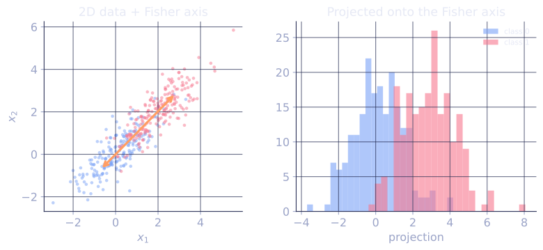
LDA can be cast as a projection problem: find the direction along which the classes are most separable, then apply a simple decision rule there. The Fisher discriminant criterion measures separability as the ratio of between-class to within-class variance, and its solution is a generalized eigenvalue problem[1]. This reframing makes LDA also a supervised dimensionality-reduction method.

The Fisher criterion

For binary classification with class means $\mu_+, \mu_-$ and shared within-class scatter $S_W$ (the LDA covariance from the previous lesson), the Fisher criterion picks a direction $w$ maximizing

The numerator $w^\top S_B w$ with $S_B = (\mu_+ - \mu_-)(\mu_+ - \mu_-)^\top$ is the between-class scatter (how far apart the class means project). The denominator is the within-class scatter along $w$ (how blurry each class projection is). The ratio is exactly "signal over noise".

The maximizer satisfies $w \propto S_W^{-1}(\mu_+ - \mu_-)$. This is the LDA direction; classifying by sign of $w^\top x + b$ on that direction recovers the LDA decision rule.

Multi-class generalization

For $K$ classes, define:

• $S_W = \sum_c \sum_{i \in c}(x_i - \mu_c)(x_i - \mu_c)^\top$ (within-class scatter).
• $S_B = \sum_c n_c (\mu_c - \bar\mu)(\mu_c - \bar\mu)^\top$ (between-class scatter, with overall mean $\bar\mu$).

The multi-class Fisher criterion maximizes $\operatorname{tr}(W^\top S_B W) / \operatorname{tr}(W^\top S_W W)$ over a projection matrix $W \in \mathbb{R}^{d \times k}$[2]. The solution is the top-$k$ eigenvectors of the generalized eigenproblem

Since $S_B$ has rank at most $K - 1$ (it lives in the span of class-mean differences), at most $K - 1$ directions have positive eigenvalues. LDA can project to at most $K - 1$ dimensions, regardless of the original $d$.

LDA versus PCA

Both produce linear projections; the difference is what they preserve:

• PCA: maximizes total variance, label-blind.
• LDA: maximizes between-class over within-class variance, label-aware.

When the most variable direction is also the most class-separating, the two agree. Often they disagree: PCA finds the noisy direction that has the most variance, while LDA finds the quieter direction that actually distinguishes classes. For visualization of labeled data, LDA's $K - 1$ projection tends to look much cleaner than PCA's.

Limits

• At most $K - 1$ dimensions. Often too few for visualization of many-class problems.
• Linear projection. Cannot capture curved manifolds. Kernel LDA and nonlinear successors exist.
• Assumes shared within-class covariance. When that fails, the criterion is suboptimal. Regularized versions help.

Check it on arrays

import numpy as np

rng = np.random.default_rng(0)

# 3-class 4D problem: classes differ along one dimension, noise in the other three
n_per = 200
mu = [np.array([+2.0, 0, 0, 0]),
      np.array([ 0.0, 0, 0, 0]),
      np.array([-2.0, 0, 0, 0])]
X, y = [], []
for c, m in enumerate(mu):
    X.append(rng.normal(loc=m, scale=1.0, size=(n_per, 4)))
    y.extend([c] * n_per)
X = np.vstack(X); y = np.array(y)

def fisher_lda(X, y):
    classes = np.unique(y)
    d = X.shape[1]
    mu_all = X.mean(axis=0)
    S_W = np.zeros((d, d)); S_B = np.zeros((d, d))
    for c in classes:
        Xc = X[y == c]
        mu_c = Xc.mean(axis=0)
        S_W += (Xc - mu_c).T @ (Xc - mu_c)
        S_B += len(Xc) * np.outer(mu_c - mu_all, mu_c - mu_all)
    # Generalized eigenproblem S_B w = lambda S_W w
    A = np.linalg.solve(S_W, S_B)
    w, V = np.linalg.eig(A)
    order = np.argsort(-w.real)
    return V[:, order].real, w[order].real

W, evals = fisher_lda(X, y)
k = 2                                                # project to 2 dims for visualization
Z = X @ W[:, :k]

# Quality: within-class variance should be much smaller than between-class
for c in np.unique(y):
    print(f"class {c}: projection mean = {Z[y == c].mean(axis=0).round(2)},  var = {Z[y == c].var(axis=0).round(3)}")

print(f"\nfirst {min(3, len(evals))} Fisher eigenvalues: {evals[:3].round(3)}")
print("Only K-1 = 2 directions are informative; the rest are essentially zero.")

# Compare to PCA: PCA's top direction is noise (since all classes have the same scale in dims 1-3)
from numpy.linalg import eigh
cov_total = np.cov(X.T)
pca_vals, pca_vecs = eigh(cov_total)
pca_top = pca_vecs[:, ::-1][:, :2]
Z_pca = X @ pca_top
sep_lda = (np.array([Z[y == c].mean(axis=0) for c in [0, 2]]).flatten() ** 2).sum()
sep_pca = (np.array([Z_pca[y == c].mean(axis=0) for c in [0, 2]]).flatten() ** 2).sum()
print(f"\nclass-mean separation in LDA 2D: {sep_lda:.3f}")
print(f"class-mean separation in PCA 2D: {sep_pca:.3f}")
print("LDA preserves class structure; PCA may not when class info is small-variance.")

LDA's eigenvalues fall off after $K - 1$, the projection lines the three classes up along one axis, and the class separation in the LDA projection beats PCA's.

Exercises

Exercise 1. For the binary Fisher criterion $J(w) = \dfrac{(w^\top(\mu_+ - \mu_-))^2}{w^\top S_W w}$, verify that the claimed maximizer $w^\star = S_W^{-1}(\mu_+ - \mu_-)$ is invariant to rescaling: show $J(cw) = J(w)$ for any nonzero scalar $c$, and explain why this means the Fisher direction is defined only up to length.

Exercise 2. Explain why the between-class scatter $S_B = \sum_c n_c (\mu_c - \bar\mu)(\mu_c - \bar\mu)^\top$ has rank at most $K - 1$, and hence why LDA can project to at most $K - 1$ dimensions.

Exercise 3 (code). Confirm the rank bound empirically. Build a $K = 4$ class problem in $d = 6$ dimensions where the class means differ, compute $S_B$, and show it has exactly $K - 1 = 3$ nonzero eigenvalues (the rest are numerically zero).

import numpy as np

rng = np.random.default_rng(0)

K, d, n_per = 4, 6, 100
means = rng.normal(size=(K, d)) * 3.0           # distinct class means
X, y = [], []
for c in range(K):
    X.append(rng.normal(loc=means[c], scale=1.0, size=(n_per, d)))
    y.extend([c] * n_per)
X = np.vstack(X); y = np.array(y)

mu_all = X.mean(axis=0)
S_B = np.zeros((d, d))
for c in range(K):
    Xc = X[y == c]
    mu_c = Xc.mean(axis=0)
    S_B += len(Xc) * np.outer(mu_c - mu_all, mu_c - mu_all)

evals = np.sort(np.abs(np.linalg.eigvalsh(S_B)))[::-1]
tol = 1e-6 * evals.max()
rank = int((evals > tol).sum())
print("eigenvalues of S_B:", evals.round(3))
print("numerical rank:", rank)
assert rank == K - 1

This closes the C4 track on instance-based and probabilistic classifiers; C5 moves to unsupervised learning.

References

- [1]Fisher, R. A. (1936). "The use of multiple measurements in taxonomic problems". Annals of Eugenics, 7(2), 179-188. The between-over-within scatter criterion and the original discriminant (doi:10.1111/j.1469-1809.1936.tb02137.x).↩
- [2]Hastie, T., Tibshirani, R., & Friedman, J. (2009). The Elements of Statistical Learning (2nd ed.). Springer. Multi-class LDA as projection and its rank limit (§4.3.3) (doi:10.1007/978-0-387-84858-7).↩