Learning and validation curves

Diagnose bias vs variance from training/validation curves over sample size and model complexity.

⏱ 22 minPrerequisites:Bias-variance decomposition

The bias-variance decomposition is a theoretical tool[1]. Learning curves and validation curves are the practical diagnostics that show, in real data, whether more data or a different model would help. Drawing these plots is the cheapest, most informative thing you can do when a model is underperforming.

Learning curve: error vs sample size

Plot training error and validation error as functions of training-set size $n$ . Both are evaluated with the same model class at each $n$ (typically with cross-validation).

Three canonical shapes:

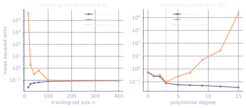
High bias (underfitting). Training and validation error converge to a high asymptote and the gap between them is small. The model is too rigid to learn the structure even with more data. Remedies: bigger model, more features, less regularization. More data will not help.

High variance (overfitting). Training error is low, validation error is much higher, and the gap is large. The model has fit the training set but not the underlying function. More data will close the gap. Remedies: more data, more regularization, simpler model[1].

Good fit. Training and validation converge to the same low asymptote. The model class is appropriate and you have enough data.

The picture tells you whether more data, more model, or different model is the next step.

Validation curve: error vs hyperparameter

Fix the dataset, vary one hyperparameter (regularization strength, polynomial degree, depth of a tree), plot training and validation error as a function of the hyperparameter.

The validation curve usually shows the bias-variance U directly:

Far on the high-regularization / low-complexity side: training and validation are both bad (high bias).
Far on the low-regularization / high-complexity side: training is great, validation is bad (high variance).
The dip in validation error is the sweet spot.

This is the visual you use to pick a hyperparameter when not running formal HPO. It also explains why the chosen hyperparameter works.

Diagnosing in practice

Workflow:

Learning curve: do I have enough data? Is the model class too simple or too complex?
Validation curve on the main hyperparameter: where is the bias-variance sweet spot?
Hold-out evaluation at the chosen configuration on a test set the search never saw.

This three-plot diagnostic is more informative than a single test number and reveals whether your investment should go into more data, more features, model complexity, or regularization.

Pitfalls

Noise in the curves at small $n$ or extreme hyperparameter values. Average over CV folds or repeated trials.
Implicit hyperparameter dependence: training a larger model needs retuning of other hyperparameters. Hold them fixed at sensible defaults, or refit them at each point on the curve (expensive).
Time / cost: drawing the full curve is many trainings. Sample sizes / hyperparameter values on a log scale.

When more data does not help

The learning curve can flatten before reaching low error. Two diagnoses:

Irreducible noise: nothing you do will get below the noise floor. The curve converges to noise variance, not zero.
Wrong features: the input variables do not contain enough signal. Adding more rows of the same data does not add information that was not there.

The cure for both is data with new content (new features, new modalities) rather than more rows of the same.

Two diagnostics: error vs training-set size (left: the train/validation gap closes as data grows) and error vs model complexity (right: the validation U-shape picks the sweet spot).

Check it on arrays

python · numpy

import numpy as np

rng = np.random.default_rng(0)

# Synthetic regression: y = sin + noise
def f_true(x): return np.sin(2 * np.pi * x)
sigma = 0.3

def gen(n, rng):
    x = rng.uniform(0, 1, n)
    return x, f_true(x) + sigma * rng.normal(size=n)

x_test = np.linspace(0, 1, 100)
y_test = f_true(x_test)

def fit_polynomial(x, y, degree):
    return np.polyfit(x, y, degree)

def predict_poly(coefs, x): return np.polyval(coefs, x)

def mse(y, y_hat): return np.mean((y - y_hat)**2)

# Learning curve: degree-9 polynomial (high variance), increase n
print("learning curve for a high-variance learner (degree-9 polynomial)")
print(f"{'n':>5}  {'train MSE':>10}  {'val MSE':>10}")
for n in [10, 20, 50, 100, 200, 500]:
    trains, vals = [], []
    for t in range(5):
        x_tr, y_tr = gen(n, np.random.default_rng(t))
        x_va, y_va = gen(200, np.random.default_rng(t + 100))
        coefs = fit_polynomial(x_tr, y_tr, degree=9)
        trains.append(mse(y_tr, predict_poly(coefs, x_tr)))
        vals.append(mse(y_va, predict_poly(coefs, x_va)))
    print(f"{n:>5}  {np.mean(trains):>10.3f}  {np.mean(vals):>10.3f}")

# Validation curve: fix n, sweep polynomial degree
print("\nvalidation curve, n = 50")
print(f"{'deg':>5}  {'train MSE':>10}  {'val MSE':>10}")
for deg in [0, 1, 3, 5, 9, 12]:
    trains, vals = [], []
    for t in range(5):
        x_tr, y_tr = gen(50, np.random.default_rng(t))
        x_va, y_va = gen(200, np.random.default_rng(t + 100))
        coefs = fit_polynomial(x_tr, y_tr, degree=deg)
        trains.append(mse(y_tr, predict_poly(coefs, x_tr)))
        vals.append(mse(y_va, predict_poly(coefs, x_va)))
    print(f"{deg:>5}  {np.mean(trains):>10.3f}  {np.mean(vals):>10.3f}")

The learning curve shows the gap shrinking as $n$ grows: high-variance learner getting cured by data. The validation curve shows the U-shape: underfitting on the left, overfitting on the right.

Exercises

Exercise 1. You draw a learning curve and find training error and validation error both plateau at MSE $\approx 0.45$ with a tiny gap between them, well above the known noise floor of $0.09$ . Diagnose the regime and say whether collecting more rows of the same data will help, justifying your answer from the curve's shape.

Solution

Step 1. A small train/validation gap with both curves converged means the model is not overfitting: it does about as poorly on data it trained on as on held-out data.

Step 2. Both curves sit at $0.45$ , far above the irreducible noise floor $0.09$ . The model cannot even fit the training data well, so the error is dominated by bias: the model class is too rigid to capture the structure.

Step 3. This is the high-bias (underfitting) regime. More rows of the same data leave the asymptote where it is, since the curves have already flattened. The remedies are a more expressive model, more or better features, or less regularization, not more data.

Exercise 2. Explain why, on a learning curve, the training error typically rises with sample size $n$ while the validation error falls, and why the two meet from opposite directions for a well-specified model.

Solution

Step 1. With very few points, a flexible model can fit the training set almost exactly, so the training error starts near zero. As $n$ grows, the same model can no longer thread every point, and its training error climbs toward the true error level.

Step 2. The validation error measures generalization. With few points the fit is unstable and overfit, so validation error starts high. As $n$ grows the estimate of the underlying function stabilizes and validation error falls toward the same true error level.

Step 3. For a correctly specified model class, both quantities converge to the irreducible noise floor: training error rising up to it, validation error falling down to it. They meet because, in the large-sample limit, the fitted model approaches the truth and in-sample and out-of-sample error coincide. A persistent gap at large $n$ is the signature of remaining variance (overfitting).

Exercise 3 (code). Make the variance-shrinks-with-data claim numerical. For a degree-5 polynomial fit on noisy sine data, measure the gap (validation MSE minus training MSE) at several sample sizes and assert it shrinks from the smallest $n$ to the largest.

Solution

python · numpy

import numpy as np

def f_true(x): return np.sin(2 * np.pi * x)
sigma = 0.3

def gen(n, rng):
    x = rng.uniform(0, 1, n)
    return x, f_true(x) + sigma * rng.normal(size=n)

def gap_at(n, degree=5, reps=20):
    gaps = []
    for t in range(reps):
        x_tr, y_tr = gen(n, np.random.default_rng(t))
        x_va, y_va = gen(400, np.random.default_rng(t + 100))
        coefs = np.polyfit(x_tr, y_tr, degree)
        train_mse = np.mean((y_tr - np.polyval(coefs, x_tr)) ** 2)
        val_mse = np.mean((y_va - np.polyval(coefs, x_va)) ** 2)
        gaps.append(val_mse - train_mse)
    return float(np.mean(gaps))

sizes = [20, 50, 100, 400]
gaps = [gap_at(n) for n in sizes]
for n, g in zip(sizes, gaps):
    print(f"n = {n:>3}:  val - train gap = {g:.4f}")
assert gaps[0] > gaps[-1]

The gap falls from about $0.087$ at $n = 20$ to about $0.004$ at $n = 400$ : the degree-5 learner is high-variance at small $n$ and the extra data closes the train/validation gap, the data-cures-variance reading of the curve.

This closes the C9 evaluation track and pillar C as a whole; the next pillar (D, Deep Learning) builds on these foundations.

References

[1]Hastie, T., Tibshirani, R., & Friedman, J. (2009). The Elements of Statistical Learning (2nd ed.). Springer. Bias-variance tradeoff and model complexity diagnostics (Ch. 7). doi:10.1007/978-0-387-84858-7↩