Probability calibration

Use reliability diagrams and Brier scores, and recalibrate with Platt scaling and isotonic regression.

⏱ 24 minPrerequisites:Classification metrics Logistic regression

A classifier is calibrated if its predicted probabilities match empirical frequencies: when it says 0.8, the event happens about 80% of the time. Many strong classifiers (random forests, SVMs, Naive Bayes) are uncalibrated, even though their rankings are excellent[1]. When probabilities feed decisions (expected-value calculations, thresholding, weighted ensembles), calibration matters as much as raw accuracy.

What calibration means

A model is perfectly calibrated if for every $p \in [0, 1]$ ,

\Pr(y = 1 \mid \hat p(x) = p) = p.

The fraction of items with predicted probability $p$ that turn out positive equals $p$ . Compute on a held-out test set by binning predictions and computing the empirical positive rate per bin.

Reliability diagrams

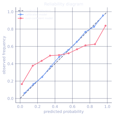
Bin the predicted probabilities (10 or 20 bins), and plot empirical positive rate (y-axis) versus mean predicted probability (x-axis) per bin. A calibrated model traces the diagonal $y = x$ .

Above the diagonal: model is underconfident (says 0.6 but the real rate is 0.8).
Below the diagonal: model is overconfident (says 0.9 but the rate is 0.7).

Most uncalibrated classifiers are overconfident at the extremes (push toward 0 and 1 too aggressively).

Brier score

A scalar summary:

\text{Brier} = \frac{1}{n}\sum_i (\hat p_i - y_i)^2.

It is the MSE of probability predictions and decomposes into reliability

resolution + uncertainty. Lower is better. Brier penalizes both poor calibration and poor accuracy.

Calibration is not ranking

The confusion worth naming: a model can rank perfectly and still be badly calibrated, because ranking only cares about the order of scores while calibration cares about their level. Take a calibrated model whose output is the true probability $p$ , and a second model that reports $\sigma(3s)$ on the same logit $s$ . The second is a monotone reshaping of the first, so it preserves order: both score the identical AUC of $0.858$ on the synthetic data below. Yet on the items the second model rates near $0.91$ , the actual positive rate is only $0.68$ , and on the items it rates above $0.95$ , the actual rate is $0.86$ . Its Brier score is $0.176$ against the calibrated $0.152$ . The ranking metric cannot see this gap; the reliability diagram and Brier score can.

Why classifiers come out miscalibrated

Random forests: probabilities are averages of leaf frequencies, which are biased toward 0.5 (a leaf with one positive and one negative example reports 50%, not the true probability).
SVMs: decision values are signed distances, not probabilities.
Naive Bayes: independent-feature assumption inflates extreme probabilities (correlated features double-count evidence).
Boosted trees: stagewise additive updates push predictions toward the extremes.

Models trained directly with log-loss (logistic regression, log-loss-tuned XGBoost, neural networks) tend to be calibrated by construction.

Platt scaling

Fit a logistic regression on top of the model's raw scores:

\hat p_{\text{cal}} = \sigma(a \cdot s + b),

with $s$ the raw score and $(a, b)$ estimated on a held-out set by log-likelihood. Two parameters; fast; works well when the miscalibration is a smooth monotonic distortion. The default for SVMs[2].

Isotonic regression

Fit a non-parametric, monotone-increasing function from raw scores to probabilities by the pool adjacent violators algorithm:

Sort scores.
For each violation of monotonicity (a higher score with a lower empirical positive rate), pool adjacent bins until monotone.

Isotonic is more flexible than Platt (can correct any monotone distortion) but needs more data and is prone to overfitting on small calibration sets.

Practical recipe

Train your classifier on the training set, leaving out a calibration set (or use cross-validation if data is scarce).
Compute raw scores or probabilities on the calibration set.
Fit Platt (small calibration set, smooth distortion) or isotonic (larger calibration set, possible non-smooth distortion).
Evaluate calibration on the test set (separate from calibration).

For deep learning, temperature scaling is the analog of Platt scaling on the logits: $\hat p = \operatorname{softmax}(z / T)$ with one scalar $T$ tuned on the calibration set. Surprisingly effective on softmax heads.

When calibration matters most

Decisions weighted by probability (expected-value, risk scoring).
Threshold tuning across cost ratios (you need probabilities to compare costs).
Ensembles that average probabilities (uncalibrated probabilities make the average garbage).
Ranking is not the issue; calibration is.

A reliability diagram plots observed frequency against predicted probability: a calibrated model hugs the diagonal, while an over-confident one flattens across it.

Check it on arrays

python · numpy

import numpy as np

rng = np.random.default_rng(0)

# Synthetic data: probability of positive depends on score
n_train, n_val, n_test = 1000, 500, 1000
def make_data(n, rng):
    s = rng.uniform(-3, 3, n)
    p = 1 / (1 + np.exp(-s))
    y = (rng.random(n) < p).astype(int)
    return s, y

s_train, y_train = make_data(n_train, rng)
s_val, y_val = make_data(n_val, rng)
s_test, y_test = make_data(n_test, rng)

# Build a miscalibrated "classifier" that amplifies the true score: a steeper
# monotone distortion makes sigmoid(miscal(s)) sit much closer to 0 / 1 than
# the true probabilities, so the classifier is overconfident at the extremes.
def miscalibrate(s): return 3.0 * s
mis_train = miscalibrate(s_train)
mis_val = miscalibrate(s_val)
mis_test = miscalibrate(s_test)

# Treat these as raw scores; convert to "probabilities" via sigmoid
def sigmoid(z): return 1 / (1 + np.exp(-z))
p_raw_test = sigmoid(mis_test)

def reliability(y, p, bins=10):
    edges = np.linspace(0, 1, bins + 1)
    bin_idx = np.digitize(p, edges) - 1
    bin_idx = np.clip(bin_idx, 0, bins - 1)
    means_p, means_y = [], []
    for b in range(bins):
        mask = bin_idx == b
        if mask.sum() > 0:
            means_p.append(p[mask].mean()); means_y.append(y[mask].mean())
    return np.array(means_p), np.array(means_y)

def brier(y, p): return np.mean((p - y)**2)

# Platt scaling on the validation set: logistic regression on raw scores
def fit_platt(scores, y, n_iter=500, lr=0.05):
    a, b = 1.0, 0.0
    for _ in range(n_iter):
        p = sigmoid(a * scores + b)
        grad_a = np.mean((p - y) * scores)
        grad_b = np.mean(p - y)
        a -= lr * grad_a; b -= lr * grad_b
    return a, b

a, b = fit_platt(mis_val, y_val)
p_platt_test = sigmoid(a * mis_test + b)

# Isotonic on the validation set (pool adjacent violators on sorted score/label pairs)
def fit_isotonic(scores, y):
    order = np.argsort(scores)
    s_sorted = scores[order]; y_sorted = y[order].astype(float)
    out = y_sorted.copy()
    weight = np.ones_like(y_sorted)
    i = 0
    while i < len(out) - 1:
        if out[i] > out[i + 1]:
            pooled = (out[i] * weight[i] + out[i + 1] * weight[i + 1]) / (weight[i] + weight[i + 1])
            out[i] = out[i + 1] = pooled
            weight[i] = weight[i + 1] = weight[i] + weight[i + 1]
            if i > 0: i -= 1
            else: i = 0
        else:
            i += 1
    return s_sorted, out

s_iso, p_iso = fit_isotonic(mis_val, y_val)
def apply_isotonic(s):
    return np.interp(s, s_iso, p_iso)
p_iso_test = apply_isotonic(mis_test)

print(f"{'method':>15}  Brier")
print(f"{'raw (sigmoid)':>15}  {brier(y_test, p_raw_test):.4f}")
print(f"{'Platt':>15}  {brier(y_test, p_platt_test):.4f}")
print(f"{'Isotonic':>15}  {brier(y_test, p_iso_test):.4f}")

Platt scaling improves Brier substantially over the raw uncalibrated probabilities; isotonic on this small validation set overfits and ends up worse, illustrating the body's caveat about isotonic needing more calibration data.

Exercises

Exercise 1. A model makes four predictions with probabilities $(0.9, 0.8, 0.3, 0.1)$ and the outcomes turn out to be $(1, 0, 0, 0)$ . Compute the Brier score by hand and identify the single prediction that hurt it most.

Solution

Step 1. The Brier score averages the squared gap between predicted probability and outcome:

\text{Brier} = \frac{1}{4}\sum_i (\hat p_i - y_i)^2.

Step 2. Compute each term: $(0.9 - 1)^2 = 0.01$ , $(0.8 - 0)^2 = 0.64$ , $(0.3 - 0)^2 = 0.09$ , $(0.1 - 0)^2 = 0.01$ .

Step 3. Average them:

\text{Brier} = \frac{0.01 + 0.64 + 0.09 + 0.01}{4} = \frac{0.75}{4} = 0.1875.

Step 4. The second prediction dominates: a confident $0.8$ on an event that did not happen contributes $0.64$ , more than five-sixths of the summed penalty. Confident mistakes are what the squared probability penalty punishes hardest.

Exercise 2. Argue that applying any strictly increasing function $g$ to a model's scores leaves its AUC unchanged but can change its Brier score. Use this to explain why a perfectly ranking model can still be badly calibrated.

Solution

Step 1. AUC is the probability that a random positive scores above a random negative: $\Pr(s_+ > s_-)$ . A strictly increasing $g$ preserves every pairwise comparison, since $s_+ > s_-$ if and only if $g(s_+) > g(s_-)$ . So the set of correctly ordered pairs is identical and AUC is unchanged.

Step 2. Brier compares the level $\hat p_i$ to $y_i$ , not the order. Replacing $\hat p_i$ by $g(\hat p_i)$ moves each prediction along the probability axis, so $\sum_i (g(\hat p_i) - y_i)^2$ generally differs from $\sum_i (\hat p_i - y_i)^2$ .

Step 3. Take a calibrated model with the true $\hat p_i$ and apply a sharpening $g$ that pushes scores toward $0$ and $1$ . The order is untouched (AUC fixed at its calibrated value), but predictions near $0.9$ now report, say, $0.97$ while the true positive rate among them is still $0.9$ . Brier rises. A model can rank flawlessly and report the wrong probability levels, which is exactly the calibration-versus-ranking gap.

Exercise 3 (code). The lesson summarizes calibration with the Brier score and reliability diagrams. A common scalar is the expected calibration error (ECE): bin the predictions, then average the gap between bin confidence and bin accuracy, weighted by bin population. Implement ECE and show that a monotone overconfident squashing, which leaves the AUC ordering intact, drives ECE up.

Solution

python · numpy

import numpy as np

rng = np.random.default_rng(0)
n = 4000
p_true = rng.uniform(0, 1, n)              # already-calibrated probabilities
y = (rng.random(n) < p_true).astype(int)

def ece(y, p, bins=10):
    edges = np.linspace(0, 1, bins + 1)
    idx = np.clip(np.digitize(p, edges) - 1, 0, bins - 1)
    total = 0.0
    for b in range(bins):
        m = idx == b
        if m.sum() > 0:
            conf = p[m].mean()             # mean predicted prob in the bin
            acc = y[m].mean()              # empirical positive rate in the bin
            total += (m.sum() / len(p)) * abs(acc - conf)
    return total

def sharpen(p):                            # strictly increasing, pushes toward 0/1
    return 1 / (1 + ((1 - p) / p) ** 3)

ece_cal = ece(y, p_true)
ece_over = ece(y, sharpen(p_true))
print(f"ECE calibrated:    {ece_cal:.4f}")
print(f"ECE overconfident: {ece_over:.4f}")
assert ece_over > ece_cal

The calibrated probabilities score about $0.014$ ECE (small, the residual binning noise), while the overconfident squashing jumps to about $0.148$ . The squashing is monotone, so it would leave AUC untouched; ECE, like the Brier score, sees the miscalibration AUC cannot.

The next lesson covers how to construct the held-out sets properly: cross-validation strategies.

References

[1]Niculescu-Mizil, A., & Caruana, R. (2005). "Predicting good probabilities with supervised learning". ICML. doi:10.1145/1102351.1102430↩
[2]Platt, J. (1999). "Probabilistic outputs for support vector machines and comparisons to regularized likelihood methods". Advances in Large Margin Classifiers. The origin of Platt scaling.↩