Regression metrics

Regression metrics share the same shape, "average penalty per residual", but the choice of penalty changes what the model optimizes for. The default MSE is great when errors are roughly Gaussian and symmetric; it is misleading when errors are heavy-tailed or asymmetric. Pick the metric that matches the cost of being wrong.

Mean squared error (MSE) and RMSE

Properties:

• The MLE for Gaussian noise (the linear-regression lesson derived this)[1].
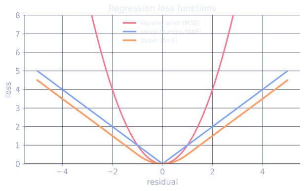
• Penalizes large errors quadratically: one residual of 10 contributes the same as 100 residuals of 1.
• Sensitive to outliers: a few extreme residuals dominate the average.
• Optimal point prediction under MSE is the conditional mean.
• RMSE has the same units as the target.

Mean absolute error (MAE)

Properties:

• Penalizes errors linearly; robust to outliers.
• Optimal point prediction is the conditional median.
• Not differentiable at zero (subgradient methods or smoothed Huber loss).

Use MAE when outliers should not dominate, or when robustness matters more than the squared-error MLE story.

R^2 (coefficient of determination)

The fraction of variance in $y$ explained by the model. Properties:

• $R^2 = 1$: perfect fit. $R^2 = 0$: model is no better than predicting $\bar y$. $R^2 < 0$: model is worse than the constant baseline.
• Scale-free, so cross-dataset comparisons are easier than with MSE.
• Inflates with model complexity on training data. Use adjusted $R^2$ on small samples.
• Holding constant the data, large $R^2$ does not mean the model is useful, only that it beats a naive mean predictor.

MAPE and other percentage metrics

Properties:

• Scale-invariant (percentage), interpretable.
• Undefined when $y_i = 0$, exploding near zero.
• Asymmetric: a forecast that is 100% too high (factor of 2) has MAPE 100%; one that is 50% too low (factor of 2 the other way) has MAPE 50%.
• Drives models to underpredict.

SMAPE (symmetric MAPE) and WAPE (weighted absolute percentage error) fix some of these issues. None are perfect; reach for percentage metrics only when business reporting demands them.

Quantile loss

For a target quantile $\tau \in (0, 1)$:

Optimizing $\ell_\tau$ gives the $\tau$-quantile predictor. Use cases:

• Asymmetric costs: under-forecasts cost more than over-forecasts (or vice versa). Quantile loss directly encodes the cost ratio.
• Prediction intervals: train separate models for the 10th and 90th quantile to get an 80% interval.
• Inventory and pricing: optimal stocking levels minimize quantile loss with $\tau$ set by the cost of stockout vs holding.

Pinball, Huber, and other robust losses

Huber loss smoothly interpolates between MSE (near zero) and MAE (far from zero), giving differentiable robustness:

Used in robust regression and as a deep-learning loss when targets have occasional outliers.

When each one misleads

• MSE / RMSE: dominated by outliers, can paint a great model as failing because of one bad point.
• MAE: indifferent to whether errors are evenly small or one huge error and the rest zero (same total).
• R^2: can be high while predictions are systematically biased.
• MAPE: explodes when targets are near zero; punishes overprediction more than underprediction.
• Quantile loss: gives no point estimate by default; tuning $\tau$ requires knowledge of the cost structure.

For most production reports, show several metrics (RMSE + MAE + a representative quantile loss), broken down by relevant slices.

Check it on arrays

import numpy as np

rng = np.random.default_rng(0)

n = 500
y = rng.normal(10, 2, n)
# Two predictors with very different error structures
y_hat_a = y + rng.normal(0, 1, n)                       # symmetric, low variance
y_hat_b = y + rng.normal(0, 0.5, n)
y_hat_b[:5] = y[:5] + 50                                # mostly excellent, 5 huge errors

def mse(y, y_hat): return np.mean((y - y_hat)**2)
def mae(y, y_hat): return np.mean(np.abs(y - y_hat))
def r2(y, y_hat): return 1 - np.sum((y - y_hat)**2) / np.sum((y - y.mean())**2)
def mape(y, y_hat): return np.mean(np.abs((y - y_hat) / y)) * 100

print(f"{'metric':>8}  {'predictor A':>12}  {'predictor B':>12}")
for name, fn in [("MSE", mse), ("RMSE", lambda y, h: np.sqrt(mse(y, h))),
                  ("MAE", mae), ("R^2", r2), ("MAPE", mape)]:
    a = fn(y, y_hat_a); b = fn(y, y_hat_b)
    print(f"{name:>8}  {a:>12.3f}  {b:>12.3f}")

print("\nPredictor B is mostly perfect but has 5 huge errors.")
print("MSE and R^2 hate it; MAE notices but is less catastrophic.")

The same predictor is judged very differently across metrics: MSE punishes the few huge errors; MAE is more forgiving.

Exercises

Exercise 1. A model produces residuals $r_i = y_i - \hat y_i$ equal to $(-2, 1, 3, -1, -1)$ on five test points. Compute the MSE, RMSE, and MAE by hand, and say which residual contributes most to each.

Exercise 2. The lesson states that the conditional median minimizes MAE. Prove the one-dimensional version: for a fixed sample $y_1, \dots, y_n$, the constant $c$ minimizing $\sum_i |y_i - c|$ is a median of the sample.

Exercise 3 (code). Confirm the two optimal-point-prediction facts at once: on a heavy-tailed sample, the constant minimizing average squared error is the mean, and the constant minimizing average absolute error is the median. Scan a dense grid of candidate constants and check each argmin against the closed-form value.

import numpy as np

rng = np.random.default_rng(0)
y = rng.normal(5, 3, 400)
y[:10] += 40                       # a heavy right tail to separate mean and median

cands = np.linspace(y.min(), y.max(), 4000)
spacing = cands[1] - cands[0]
mse = np.array([np.mean((y - c) ** 2) for c in cands])
mae = np.array([np.mean(np.abs(y - c)) for c in cands])

c_mse = cands[mse.argmin()]
c_mae = cands[mae.argmin()]
print(f"argmin MSE = {c_mse:.4f}  vs mean   = {y.mean():.4f}")
print(f"argmin MAE = {c_mae:.4f}  vs median = {np.median(y):.4f}")

assert abs(c_mse - y.mean()) < spacing
assert abs(c_mae - np.median(y)) < spacing

The next lesson tackles a different metric concern: are the predicted probabilities believable?

References

- [1]Hastie, T., Tibshirani, R., & Friedman, J. (2009). The Elements of Statistical Learning (2nd ed.). Springer. Squared-error loss, robust losses, and the bias-variance view of regression error. doi:10.1007/978-0-387-84858-7↩