 AI Knowledge Tree
Classification metrics
Define precision, recall, F1, ROC curves, and AUC; choose the metric that matches the cost structure.
Accuracy is a terrible metric for most real classification problems: under class imbalance, a constant predictor can hit 99% accuracy and be useless. The standard alternatives, precision, recall, F1, ROC-AUC, PR-AUC, all emphasize different aspects of model behavior. Picking the right one means matching the metric to the cost of mistakes in your problem.
The confusion matrix
For binary classification with a threshold producing predicted positives and negatives:
| Predicted + | Predicted - | |
|---|---|---|
| Actual + | TP | FN |
| Actual - | FP | TN |
- TP = true positives
- FP = false positives
- FN = false negatives
- TN = true negatives
Every metric below is a function of these four counts.
Accuracy and its failure on imbalance
.
The fatal flaw: on a 99/1 imbalanced dataset, predicting "always 0" gives 99% accuracy. Use accuracy only when classes are roughly balanced and false positives cost the same as false negatives.
Precision and recall
- Precision: of the items I flagged positive, how many actually were? High precision = low false alarms.
- Recall (sensitivity, true positive rate): of the actually positive items, how many did I catch? High recall = few misses.
Precision and recall are in tension: lowering the threshold catches more positives (recall up) at the cost of more false positives (precision down).
F1 score
The harmonic mean of precision and recall:
F1 collapses precision and recall into one number with equal weight. F1 is useful as a single metric to optimize, especially under imbalance, but it hides the precision-recall tradeoff. F generalizes: favors precision, favors recall[2].
ROC curve and AUC
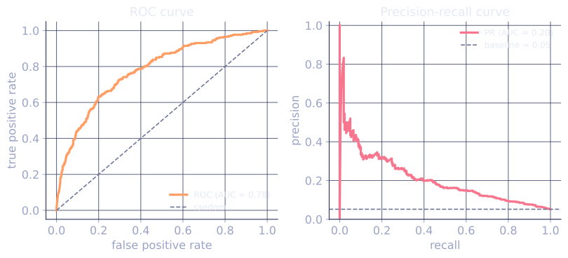
Vary the classifier's threshold and trace TPR (recall) against FPR (). The result is the ROC curve. The area under the ROC curve (AUC-ROC) is the probability that a randomly chosen positive gets a higher score than a randomly chosen negative[1].
Properties:
- AUC = 1: perfect ranking.
- AUC = 0.5: random.
- AUC < 0.5: worse than random (flip your scores).
AUC is threshold-independent: it measures ranking quality, not calibration or operating point. Convenient when the threshold will be chosen later by downstream cost.
Precision-recall curve and PR-AUC
Plot precision vs recall as the threshold varies. The PR-AUC is the area under it. Important property:
- PR curves are sensitive to class imbalance in a way ROC is not. On severely imbalanced datasets, ROC-AUC can look great even when the classifier is useless in the relevant operating range.
Use PR-AUC for imbalanced positive classes (rare positives): fraud detection, anomaly detection, retrieval. Use ROC-AUC for balanced problems or when you care about overall ranking quality.
Multi-class extensions
- Macro-average: compute the metric per class, then average. Treats every class equally regardless of size.
- Micro-average: aggregate TP/FP/FN/TN across all classes, then compute the metric. Dominated by frequent classes.
- Weighted-average: per-class metric weighted by class frequency.
Pick macro for fair-across-class treatment, micro for overall accuracy, weighted when classes are imbalanced but treated proportionally.
When to use what
| Problem | Metric |
|---|---|
| Balanced classes, equal costs | Accuracy |
| Imbalanced positives | PR-AUC, recall at high precision |
| Imbalanced negatives, ranking matters | ROC-AUC |
| Cost-sensitive (FP and FN have known costs) | Optimize expected cost directly |
| Need a single number | F1 or F |
| Multi-class fairness across classes | Macro-F1 |
The honest answer is usually "report several and use the one that matches the real cost structure of mistakes". A single number rarely tells the whole story.
Check it on arrays
import numpy as np

rng = np.random.default_rng(0)

# Imbalanced binary problem: 5% positive class
n = 5000
y = (rng.random(n) < 0.05).astype(int)
# Synthetic scores: noisy version of y
scores = y + 0.7 * rng.normal(size=n)

def confusion(y_true, y_pred):
    tp = int(((y_pred == 1) & (y_true == 1)).sum())
    fp = int(((y_pred == 1) & (y_true == 0)).sum())
    fn = int(((y_pred == 0) & (y_true == 1)).sum())
    tn = int(((y_pred == 0) & (y_true == 0)).sum())
    return tp, fp, fn, tn

def metrics_at_threshold(y_true, scores, thr):
    y_pred = (scores >= thr).astype(int)
    tp, fp, fn, tn = confusion(y_true, y_pred)
    prec = tp / max(tp + fp, 1)
    rec = tp / max(tp + fn, 1)
    f1 = 2 * prec * rec / max(prec + rec, 1e-9)
    return prec, rec, f1, (tp + tn) / max(n, 1)

for thr in [0.0, 0.5, 1.0, 1.5]:
    prec, rec, f1, _ = metrics_at_threshold(y, scores, thr)
    acc = ((scores >= thr).astype(int) == y).mean()
    print(f"thr={thr:>4.1f}: precision={prec:.3f}, recall={rec:.3f}, F1={f1:.3f}, accuracy={acc:.3f}")

def auc_roc(y_true, scores):
    # Sort by descending score; trace TPR, FPR
    order = np.argsort(-scores)
    y_sorted = y_true[order]
    tpr = np.cumsum(y_sorted) / max(y_sorted.sum(), 1)
    fpr = np.cumsum(1 - y_sorted) / max((1 - y_sorted).sum(), 1)
    # Trapezoidal area
    integrate = np.trapezoid if hasattr(np, "trapezoid") else np.trapz
    return integrate(tpr, fpr)

def auc_pr(y_true, scores):
    order = np.argsort(-scores)
    y_sorted = y_true[order]
    tp = np.cumsum(y_sorted)
    fp = np.cumsum(1 - y_sorted)
    precision = tp / np.maximum(tp + fp, 1)
    recall = tp / max(y_true.sum(), 1)
    integrate = np.trapezoid if hasattr(np, "trapezoid") else np.trapz
    return integrate(precision, recall)

print(f"\nROC-AUC: {auc_roc(y, scores):.3f}")
print(f"PR-AUC:  {auc_pr(y, scores):.3f}")

# An always-zero predictor: 95% accuracy but 0% recall
print(f"\ntrivial all-zero classifier: accuracy={1 - y.mean():.3f}, recall=0.000")
The always-zero classifier has high accuracy but useless recall on the imbalanced data; PR-AUC reflects the actual ranking quality more honestly than accuracy.
Exercises
Exercise 1. A spam filter is evaluated on 1000 emails. It produces the confusion counts , , , . Compute its precision, recall, , and accuracy by hand, and explain which number a user who hates losing real mail to the spam folder should care about most.
Solution
Step 1. Precision is the fraction of flagged-spam that is truly spam:
Step 2. Recall is the fraction of true spam that was caught:
Step 3. is the harmonic mean:
Step 4. Accuracy is the overall correct fraction:
Step 5. A real email sent to the spam folder is a false positive. The user who hates that cares about precision (here , meaning one in five flagged emails is actually legitimate), not the headline accuracy, which is inflated by the many easy true negatives.
Exercise 2. Show that can never exceed the larger of precision and recall, and equals both only when precision recall. Use this to argue why is a conservative single-number summary.
Solution
Step 1. Write for precision and for recall, both in . The harmonic mean is
Step 2. Compare to . Assume without loss of generality , so . Then
where the inequality uses (since ). So .
Step 3. Equality in Step 2 needs , that is . When , . So touches the larger value only on the diagonal .
Step 4. Whenever precision and recall disagree, sits strictly below the larger of them and is pulled toward the smaller. This is the conservative behavior of the harmonic mean: a model cannot earn a high by being excellent on one axis and poor on the other.
Exercise 3 (code). The lesson computes AUC by a trapezoidal sweep of the ROC curve. The probabilistic definition says AUC equals the probability a random positive outscores a random negative, which is the Mann-Whitney rank statistic. Implement the rank-based AUC and verify it matches the trapezoidal sweep to three decimals on synthetic scores.
Solution
import numpy as np

rng = np.random.default_rng(0)
n = 2000
y = (rng.random(n) < 0.3).astype(int)
scores = y + 0.8 * rng.normal(size=n)

def auc_rank(y, s):
    # Mann-Whitney: (sum of positive ranks - n_pos(n_pos+1)/2) / (n_pos n_neg)
    order = np.argsort(s)
    ranks = np.empty(len(s))
    ranks[order] = np.arange(1, len(s) + 1)
    n_pos = int((y == 1).sum())
    n_neg = int((y == 0).sum())
    sum_ranks_pos = ranks[y == 1].sum()
    return (sum_ranks_pos - n_pos * (n_pos + 1) / 2) / (n_pos * n_neg)

def auc_trap(y, s):
    order = np.argsort(-s)
    ys = y[order]
    tpr = np.cumsum(ys) / max(ys.sum(), 1)
    fpr = np.cumsum(1 - ys) / max((1 - ys).sum(), 1)
    integrate = np.trapezoid if hasattr(np, "trapezoid") else np.trapz
    return integrate(tpr, fpr)

a_rank = auc_rank(y, scores)
a_trap = auc_trap(y, scores)
print(f"rank AUC: {a_rank:.4f}   trapezoidal AUC: {a_trap:.4f}")
assert np.isclose(a_rank, a_trap, atol=1e-3)
Both routes land on : the rank-based count of positive-over-negative pairs is the same number the trapezoidal ROC integral computes, which is why AUC is called a ranking metric.
The next lesson covers the regression analogs.
References
- [1]Fawcett, T. (2006). "An introduction to ROC analysis". Pattern Recognition Letters, 27(8), 861-874. doi:10.1016/j.patrec.2005.10.010↩
- [2]Powers, D. M. W. (2011). "Evaluation: from precision, recall and F-measure to ROC, informedness, markedness and correlation". Journal of Machine Learning Technologies, 2(1), 37-63.↩