Hard-margin SVM

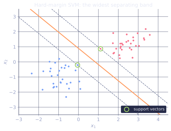
The perceptron settles for any separating hyperplane. The support vector machine (SVM) demands a particular one: the hyperplane that maximizes the distance to the nearest training point[1]. This maximum-margin formulation turns into a convex quadratic program, with a clean geometric story.

The margin

For a hyperplane $\{x : w^\top x + b = 0\}$ with unit normal $\hat w = w / \lVert w \rVert$, the signed distance from a point $x$ to the hyperplane is $(w^\top x + b)/\lVert w\rVert$.

For labels $y_i \in \{-1, +1\}$, the geometric margin of a point is

It is positive when the point is on the correct side, negative otherwise. The margin of the dataset is $\gamma = \min_i \gamma_i$, the distance to the closest point.

The maximum-margin problem

Maximizing the dataset margin subject to all points being correctly classified:

The objective is invariant under positive scaling of $(w, b)$, so fix the scale by requiring the closest point to satisfy $y_i(w^\top x_i + b) = 1$. Then $\gamma = 1/\lVert w\rVert$, and maximizing $\gamma$ is minimizing $\lVert w\rVert$.

The scaling invariance is worth pinning down, because two "margins" are easy to conflate. The functional margin $y_i(w^\top x_i + b)$ is the raw score; the geometric margin divides it by $\lVert w\rVert$ and is the actual distance. Take the hyperplane $w = (1, 0)$, $b = 0$ and a point at $x = (2, 0)$: the functional margin is $2$ and the geometric margin is $2/\lVert w\rVert = 2$, a real distance of two units. Rescale to $w = (5, 0)$ (same hyperplane, the line $x_1 = 0$ is unchanged): the functional margin balloons to $10$, but the geometric margin is $10/5 = 2$, unchanged. Only the geometric margin means anything; the functional one can be inflated to any value by scaling $w$. Pinning the closest functional margin to $1$ removes that freedom, after which $\gamma = 1/\lVert w\rVert$ reads off the geometric margin directly: $\lVert w\rVert = 2$ is a margin of $0.5$, $\lVert w\rVert = 0.5$ is a margin of $2$.

The hard-margin SVM

The factor $\tfrac{1}{2}$ is for derivative cleanness. The objective is convex quadratic and the constraints are affine, so this is a convex quadratic program (QP). It has a unique global solution whenever the data are linearly separable; otherwise the constraint set is empty and the problem is infeasible (which is what the next lesson fixes with slack).

KKT conditions and support vectors

Form the Lagrangian with multipliers $\alpha_i \ge 0$:

Stationarity gives

The first equation says the optimal $w$ is a linear combination of the training points (with $y_i$-signed weights). Complementary slackness says $\alpha_i = 0$ unless the margin constraint is tight, i.e. $y_i(w^\top x_i + b) = 1$.

Points with $\alpha_i > 0$ sit exactly on the margin boundary. They are the support vectors, and they are the only data points that contribute to $w$. Everything else is irrelevant to the classifier; this is the SVM's celebrated sparsity-in-examples property[2].

What hard-margin can't handle

Three failure modes drive the next lessons:

• Nonseparable data. No feasible $(w, b)$ exists. Soft margin (next lesson) introduces slack.
• Outliers near the boundary. A single bad label forces the entire hyperplane to compensate, hurting generalization. Soft margin also fixes this.
• Nonlinear separators. The decision boundary is forced to be linear in $x$. The kernel trick lifts the problem to a higher-dimensional space where linear separation suffices.

Check it on arrays

import numpy as np

rng = np.random.default_rng(0)

# Linearly separable 2D data
n_per = 30
X_pos = rng.normal(loc=[2.5, 1.0], scale=0.6, size=(n_per, 2))
X_neg = rng.normal(loc=[-1.0, -1.0], scale=0.6, size=(n_per, 2))
X = np.vstack([X_pos, X_neg])
y = np.array([1.0] * n_per + [-1.0] * n_per)

# Hard-margin SVM via projected gradient on the dual:
#   max sum(alpha) - 0.5 alpha^T (y y^T * K) alpha   s.t. alpha >= 0, sum(y * alpha) = 0
def hard_margin_dual(X, y, lr=1e-3, steps=20000):
    K = X @ X.T                           # linear kernel
    Q = (y[:, None] * y[None, :]) * K
    n = len(y)
    alpha = np.zeros(n)
    for _ in range(steps):
        grad = 1 - Q @ alpha
        alpha = alpha + lr * grad
        alpha = np.maximum(alpha, 0)      # alpha >= 0
        # project to satisfy sum(y * alpha) = 0
        alpha -= y * (y @ alpha) / (y @ y)
        alpha = np.maximum(alpha, 0)
    return alpha

alpha = hard_margin_dual(X, y)

# Recover w and b from the support vectors
w = (alpha * y) @ X
sv_idx = np.where(alpha > 1e-4)[0]
print(f"support vectors: {len(sv_idx)} / {len(y)}")
b = np.mean(y[sv_idx] - X[sv_idx] @ w)
print(f"w = {w}, b = {b:.3f}")

# Margin and accuracy
margin = 1.0 / np.linalg.norm(w)
print(f"geometric margin = {margin:.3f}")
acc = np.mean(np.sign(X @ w + b) == y)
print(f"training accuracy = {acc:.3f}")

# The decision boundary passes between the two classes
print("min positive margin:", np.min(y * (X @ w + b)))

The dual ascent identifies a handful of support vectors; the recovered weight vector classifies every training point correctly with a positive margin.

Exercises

Exercise 1. Two points lie on a line through the origin: $x_+ = (1, 1)$ with $y_+ = +1$ and $x_- = (-1, -1)$ with $y_- = -1$. Find the hard-margin solution $(w, b)$ and the geometric margin, by enforcing that both points sit on the margin boundary.

Exercise 2. From the stationarity condition $w = \sum_i \alpha_i y_i x_i$ and $\sum_i \alpha_i y_i = 0$, prove that the squared norm equals $\lVert w\rVert^2 = \sum_i \alpha_i$, so the squared margin is $1/\sum_i \alpha_i$. (Use that for support vectors $y_i(w^\top x_i + b) = 1$.)

Exercise 3 (code). Take the two points of Exercise 1, run the projected- gradient dual ascent, and confirm it recovers $w = (1/2, 1/2)$, $b = 0$, a margin of $\sqrt2$, and equal multipliers $\alpha_+ = \alpha_-$.

import numpy as np

X = np.array([[1.0, 1.0], [-1.0, -1.0]])
y = np.array([1.0, -1.0])

def hard_margin_dual(X, y, lr=1e-3, steps=50000):
    K = X @ X.T
    Q = (y[:, None] * y[None, :]) * K
    alpha = np.zeros(len(y))
    for _ in range(steps):
        grad = 1 - Q @ alpha
        alpha = np.maximum(alpha + lr * grad, 0)
        alpha -= y * (y @ alpha) / (y @ y)     # project onto sum(y*alpha)=0
        alpha = np.maximum(alpha, 0)
    return alpha

alpha = hard_margin_dual(X, y)
w = (alpha * y) @ X
sv = alpha > 1e-4
b = np.mean(y[sv] - X[sv] @ w)
margin = 1.0 / np.linalg.norm(w)

print(f"w = {w}, b = {b:.3f}, margin = {margin:.4f}, alpha = {alpha}")
assert np.allclose(w, [0.5, 0.5], atol=1e-2)
assert np.isclose(margin, np.sqrt(2), atol=1e-2)
assert np.isclose(alpha[0], alpha[1], atol=1e-3)   # symmetric multipliers

The next lesson relaxes the hard constraints with slack variables so the SVM survives noisy and nonseparable data.

References

- [1]Boser, B. E., Guyon, I. M., & Vapnik, V. N. (1992). "A training algorithm for optimal margin classifiers". COLT. Introduces the maximum-margin classifier (doi:10.1145/130385.130401).↩
- [2]Vapnik, V. N. (1998). Statistical Learning Theory. Wiley. The foundational treatment of margins, support vectors, and generalization.↩