Gaussian process regression

A Gaussian process is a probability distribution over functions[1]. Place a GP prior on the unknown regression function, condition on observed data, and the posterior is again a Gaussian (over function values), with a closed-form mean and variance at every test point. GPs marry kernels with full Bayesian machinery, and they are the engine of Bayesian optimization.

A distribution over functions

Define a GP $f \sim \mathcal{GP}(m, k)$ by:

• a mean function $m: \mathcal{X} \to \mathbb{R}$ (often $m \equiv 0$),
• a covariance (kernel) function $k: \mathcal{X} \times \mathcal{X} \to \mathbb{R}$ that is symmetric and positive semidefinite.

Drawing from the GP at any finite set of inputs $X_\star = (x_{\star 1}, \dots, x_{\star m})$ gives a finite-dimensional Gaussian vector:

with $K(X_\star, X_\star)_{ij} = k(x_{\star i}, x_{\star j})$. A function draw is a random vector at any chosen evaluation grid.

Conditioning on data

Suppose observations are $y_i = f(x_i) + \varepsilon_i$ with $\varepsilon_i \sim \mathcal{N}(0, \sigma_n^2)$. Stack training inputs into $X$ and outputs into $\mathbf{y}$. By the Gaussian conditional formula, the joint distribution of $(\mathbf{y}, \mathbf{f}_\star)$ is Gaussian, and conditioning on $\mathbf{y}$ gives the posterior:

with

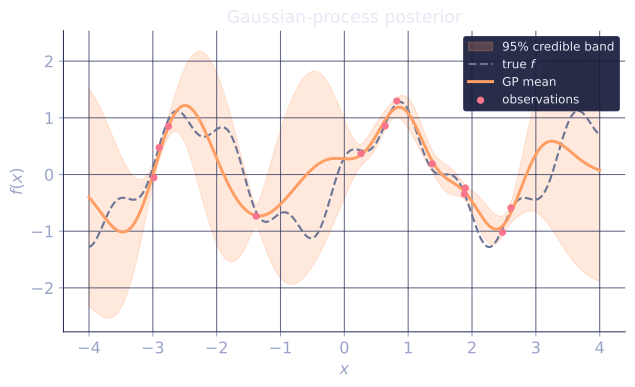
The posterior mean is a linear combination of training outputs, with weights depending on the kernel. The posterior variance shrinks where training data is dense and grows where it is sparse, with no extra effort: calibrated uncertainty falls out for free.

Hyperparameters via marginal likelihood

The kernel $k$ has its own hyperparameters (e.g. RBF length scale $\ell$ and amplitude $\sigma_f$). Choose them by maximizing the log marginal likelihood:

The first term rewards data fit; the second penalizes model complexity (the log-determinant grows when the kernel implies high flexibility). This is the Bayesian Occam's razor at work, with no separate validation set needed for hyperparameter selection[2].

Costs and scalability

The GP posterior costs $O(n^3)$ to compute (the inversion of $K_{XX} + \sigma_n^2 I$) and $O(n^2)$ memory. This is manageable up to a few thousand points and gets prohibitive past tens of thousands. Standard fixes:

• Sparse approximations (inducing points, FITC, VFE).
• Low-rank kernel approximations (Nyström, random Fourier features).
• Structured kernels (e.g. product kernels on grids, exploited by Kronecker tricks).

GPs are not the right tool for very large datasets; they are the right tool when each data point is expensive and uncertainty matters.

Use cases

• Bayesian optimization: the GP is the surrogate model whose posterior variance drives exploration (see the A3 lesson).
• Spatial statistics (kriging): the original application, predicting mineral concentrations from a few drill holes.
• Hyperparameter response surfaces: model training accuracy as a function of hyperparameters and use the GP posterior to decide what to try next.
• Calibrated regression: any setting where decision-quality predictive variance matters more than raw accuracy.

Check it on arrays

import numpy as np

rng = np.random.default_rng(0)

# Toy 1D regression
def f_true(x): return np.sin(2 * x) + 0.3 * np.cos(7 * x)
n = 12
x_train = np.sort(rng.uniform(-3, 3, n))[:, None]
y_train = f_true(x_train).ravel() + 0.1 * rng.normal(size=n)

x_test = np.linspace(-4, 4, 200)[:, None]

def rbf(X1, X2, ell=1.0, sigma_f=1.0):
    d2 = np.sum(X1**2, 1)[:, None] + np.sum(X2**2, 1) - 2 * X1 @ X2.T
    return sigma_f**2 * np.exp(-0.5 * d2 / ell**2)

def gp_posterior(x_train, y_train, x_test, ell, sigma_f, sigma_n):
    Kxx = rbf(x_train, x_train, ell, sigma_f) + sigma_n**2 * np.eye(len(x_train))
    Kxs = rbf(x_train, x_test, ell, sigma_f)
    Kss = rbf(x_test, x_test, ell, sigma_f) + 1e-8 * np.eye(len(x_test))
    L = np.linalg.cholesky(Kxx)
    alpha = np.linalg.solve(L.T, np.linalg.solve(L, y_train))
    v = np.linalg.solve(L, Kxs)
    mu = Kxs.T @ alpha
    cov = Kss - v.T @ v
    return mu, np.sqrt(np.maximum(np.diag(cov), 0))

ell, sigma_f, sigma_n = 0.5, 1.0, 0.1
mu, sd = gp_posterior(x_train, y_train, x_test, ell, sigma_f, sigma_n)

# Reality check: posterior mean is close to the truth and uncertainty grows away from data
err_at_data = np.linalg.norm(gp_posterior(x_train, y_train, x_train, ell, sigma_f, sigma_n)[0] - y_train) / len(y_train)
print(f"in-sample RMSE: {err_at_data:.3f}")
print(f"posterior sd at first  test point: {sd[0]:.3f}  (far from data)")
print(f"posterior sd at center test point: {sd[len(sd) // 2]:.3f}  (near data)")
print(f"95% CI covers truth? "
      f"{np.mean(np.abs(mu - f_true(x_test).ravel()) <= 1.96 * sd):.2%}")

# Log marginal likelihood as a function of length scale
ells = np.linspace(0.1, 2.0, 25)
lmls = []
for L in ells:
    Kxx = rbf(x_train, x_train, L, sigma_f) + sigma_n**2 * np.eye(len(x_train))
    sign, logdet = np.linalg.slogdet(Kxx)
    alpha = np.linalg.solve(Kxx, y_train)
    lml = -0.5 * y_train @ alpha - 0.5 * logdet - 0.5 * len(x_train) * np.log(2 * np.pi)
    lmls.append(lml)
best_ell = ells[int(np.argmax(lmls))]
print(f"best ell by marginal likelihood: {best_ell:.2f}")

The GP posterior fits the training data, gives tight uncertainty near the samples and wide uncertainty far from them, and the marginal likelihood picks a reasonable length scale.

Exercises

Exercise 1. A noiseless GP ($\sigma_n^2 = 0$) has a single training point $x_1 = 0$ with $y_1 = 1$, and an RBF kernel with $\sigma_f = 1$, $\ell = 1$, so $k(x, x') = \exp(-\tfrac12 (x - x')^2)$. Compute the posterior mean and variance at a test point $x_\star$, and evaluate them at $x_\star = 0$.

Exercise 2. In the log marginal likelihood $-\tfrac12 \mathbf{y}^\top A^{-1}\mathbf{y} - \tfrac12 \log\det A - \tfrac{n}{2}\log(2\pi)$ with $A = K_{XX} + \sigma_n^2 I$, explain why the $-\tfrac12\log\det A$ term acts as a complexity penalty. (Consider how $\det A$ changes when the kernel is made more flexible.)

Exercise 3 (code). On a 1D toy regression, verify that a near-noiseless GP interpolates its training points (posterior mean matches $y$, posterior standard deviation near zero at training inputs), and that the posterior standard deviation is larger at a point far from all data than at a point near the data.

import numpy as np

rng = np.random.default_rng(0)

def f_true(x):
    return np.sin(2 * x) + 0.3 * np.cos(7 * x)

n = 12
x_train = np.sort(rng.uniform(-3, 3, n))[:, None]
y_train = f_true(x_train).ravel() + 0.1 * rng.normal(size=n)

def rbf(X1, X2, ell=1.0, sigma_f=1.0):
    d2 = np.sum(X1**2, 1)[:, None] + np.sum(X2**2, 1) - 2 * X1 @ X2.T
    return sigma_f**2 * np.exp(-0.5 * d2 / ell**2)

def gp_posterior(x_train, y_train, x_test, ell, sigma_f, sigma_n):
    Kxx = rbf(x_train, x_train, ell, sigma_f) + sigma_n**2 * np.eye(len(x_train))
    Kxs = rbf(x_train, x_test, ell, sigma_f)
    Kss = rbf(x_test, x_test, ell, sigma_f) + 1e-8 * np.eye(len(x_test))
    L = np.linalg.cholesky(Kxx)
    alpha = np.linalg.solve(L.T, np.linalg.solve(L, y_train))
    v = np.linalg.solve(L, Kxs)
    mu = Kxs.T @ alpha
    cov = Kss - v.T @ v
    return mu, np.sqrt(np.maximum(np.diag(cov), 0))

# Near-noiseless GP interpolates the training points
mu_tr, sd_tr = gp_posterior(x_train, y_train, x_train, 0.5, 1.0, 1e-6)
assert np.allclose(mu_tr, y_train, atol=1e-3)
assert sd_tr.max() < 1e-2

# Uncertainty grows away from data
_, sd_far = gp_posterior(x_train, y_train, np.array([[10.0]]), 0.5, 1.0, 0.1)
_, sd_near = gp_posterior(x_train, y_train, x_train[n // 2:n // 2 + 1], 0.5, 1.0, 0.1)
print(f"sd far from data: {sd_far[0]:.3f}, sd near data: {sd_near[0]:.3f}")
assert sd_far[0] > sd_near[0]

This closes the C2 margin-and-kernels track; the next subsection switches to a very different inductive bias: trees that split the input space along axis-aligned cuts.

References

- [1]Rasmussen, C. E., & Williams, C. K. I. (2006). Gaussian Processes for Machine Learning. MIT Press. The canonical reference for GP regression, the posterior formulas, and scalable approximations.↩
- [2]Bishop, C. M. (2006). Pattern Recognition and Machine Learning. Springer. §6.4 derives the GP marginal likelihood and the Bayesian Occam's razor.↩