RBF, polynomial, and string kernels

The kernel trick is general; in practice a handful of kernels do most of the work. The RBF is the universal default; the polynomial captures explicit interactions; string kernels lift the framework to non-vector inputs like text and biological sequences[1]. Knowing each kernel's hyperparameters and failure modes is most of using kernel methods well.

The RBF (Gaussian) kernel

Properties:

• Implicit infinite-dimensional features. The Taylor expansion of $\exp$ shows $\phi$ has infinitely many components.
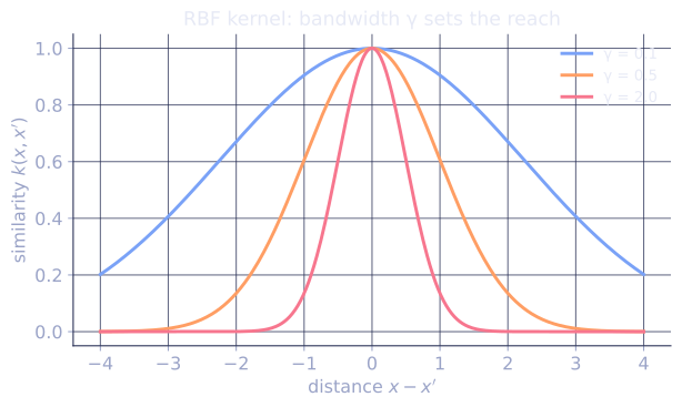
• Locality. $k(x, x') \to 0$ as $\lVert x - x'\rVert \to \infty$, so each training point influences a region of size $\sim 1/\sqrt\gamma$.
• One hyperparameter, $\gamma$ (or $\sigma$ with $\gamma = 1/(2\sigma^2)$). Large $\gamma$: tiny influence radius, complex boundaries, risk of overfitting. Small $\gamma$: huge influence radius, smooth boundaries, risk of underfitting.

RBF is the safe first choice when you have no specific structural knowledge about the data[2].

The polynomial kernel

Hyperparameters: degree $p$, scale $\gamma$, offset $c$.

The feature map contains all monomials in the features up to degree $p$. For $p = 2$, $c = 1$ and 2D input, $\phi$ has components $\{1, \sqrt 2 x_1, \sqrt 2 x_2, x_1^2, x_2^2, \sqrt 2 x_1 x_2\}$ (verified in the previous lesson). Good when explicit feature interactions matter and when the relevant degree is small. Bad when the degree is large: the Gram matrix becomes ill-conditioned and the model overfits.

String kernels

For non-vector inputs, define the inner product directly. For sequences (text, DNA, code), the spectrum kernel counts how many length-$k$ substrings two sequences share:

where $\#u(s)$ counts occurrences of substring $u$ in $s$. The induced feature map is the histogram of $k$-mers; the kernel is the dot product of histograms, computed in time linear in the lengths via suffix-array data structures.

Variants: gap-weighted string kernels allow non-contiguous substrings with length-decaying weights; mismatch kernels allow approximate matches. These were the dominant approach to sequence classification before deep learning.

Combining kernels: practical recipes

The composition rules from the previous lesson let you build problem-specific kernels:

• Multiple data sources. Sum kernels from different modalities, $k = k_{\text{text}} + k_{\text{image}}$, to combine them.
• Sparse + smooth. Sum a polynomial kernel (captures explicit interactions) and an RBF (captures smooth residual structure).
• Normalized kernels. Replace $k(x, x')$ with $k(x, x')/\sqrt{k(x,x)\, k(x',x')}$ to make the kernel scale-invariant.

Picking hyperparameters

Cross-validate over a grid:

• RBF: jointly sweep $C$ (regularization) and $\gamma$ (bandwidth), log-scale.
• Polynomial: degrees 2 or 3 are typical; very rarely above 5.
• Composite: validate the mixture weights too.

A median-distance heuristic for RBF: set $\gamma = 1/\operatorname{median}_{i \ne j}\lVert x_i - x_j\rVert^2$. It is usually within an order of magnitude of the cross-validated optimum and is a cheap starting point.

Check it on arrays

import numpy as np

rng = np.random.default_rng(0)

# Sample data
n = 100
X = rng.normal(size=(n, 4))

def rbf(X1, X2, gamma):
    d2 = np.sum(X1**2, 1)[:, None] + np.sum(X2**2, 1) - 2 * X1 @ X2.T
    return np.exp(-gamma * d2)

def poly(X1, X2, gamma=1.0, c=1.0, p=3):
    return (gamma * X1 @ X2.T + c)**p

# Both Gram matrices are PSD
K_rbf = rbf(X, X, gamma=0.5)
K_poly = poly(X, X, p=3)
print(f"RBF min eig:  {np.min(np.linalg.eigvalsh(K_rbf)):.3e}")
print(f"poly min eig: {np.min(np.linalg.eigvalsh(K_poly)):.3e}")

# Median-distance heuristic for gamma
from itertools import combinations
ij = list(combinations(range(n), 2))
dists2 = [np.sum((X[i] - X[j])**2) for i, j in ij[:5000]]
gamma_med = 1 / np.median(dists2)
print(f"median-distance gamma: {gamma_med:.3f}")

# Sum kernel: K = K_rbf + K_poly is still PSD
K_sum = K_rbf + K_poly
print(f"sum kernel min eig: {np.min(np.linalg.eigvalsh(K_sum)):.3e}")

# String kernel (spectrum kernel, k=2): count shared bigrams in short strings
def spectrum_kernel(s, t, k=2):
    def kmers(x):
        bag = {}
        for i in range(len(x) - k + 1):
            bag[x[i:i+k]] = bag.get(x[i:i+k], 0) + 1
        return bag
    a, b = kmers(s), kmers(t)
    return sum(a[u] * b.get(u, 0) for u in a)

strings = ["statistics", "stochastic", "statistician", "biology"]
n_str = len(strings)
K_str = np.array([[spectrum_kernel(s, t, k=2) for t in strings] for s in strings], dtype=float)
print("\nstring-kernel Gram (bigram counts):")
print(K_str.astype(int))

All three Gram matrices come out PSD; the median-distance heuristic gives a reasonable starting $\gamma$; the bigram spectrum kernel correctly puts "statistics" closer to its morphological neighbors than to "biology".

Exercises

Exercise 1. Compute the bigram ($k = 2$) spectrum kernel $k(s, t)$ by hand for the strings $s =$ "aba" and $t =$ "abab", and for $k(s, s)$.

Exercise 2. The product $k(x, x') = k_1(x, x')\, k_2(x, x')$ of two valid kernels is again a valid kernel. Take $k_1 = k_2 = x^\top x'$ on $\mathbb{R}^2$ and exhibit the explicit feature map of the product, confirming it contains the degree-2 monomials.

Exercise 3 (code). Take an RBF Gram matrix and a degree-3 polynomial Gram matrix on random data. Verify that their sum is still positive semidefinite, and that the RBF kernel, after normalization $k(x,x')/\sqrt{k(x,x)\,k(x',x')}$, has a unit diagonal and entries within $[-1, 1]$.

import numpy as np

rng = np.random.default_rng(0)
X = rng.normal(size=(50, 4))

def rbf(X1, X2, gamma):
    d2 = np.sum(X1**2, 1)[:, None] + np.sum(X2**2, 1) - 2 * X1 @ X2.T
    return np.exp(-gamma * d2)

def poly(X1, X2, gamma=1.0, c=1.0, p=3):
    return (gamma * X1 @ X2.T + c)**p

K_rbf = rbf(X, X, gamma=0.5)
K_poly = poly(X, X, p=3)

# Sum of two valid kernels stays PSD
K_sum = K_rbf + K_poly
assert np.linalg.eigvalsh(K_sum).min() > -1e-8

# Normalized kernel: unit diagonal, entries in [-1, 1]
d = np.sqrt(np.diag(K_rbf))
K_norm = K_rbf / np.outer(d, d)
assert np.allclose(np.diag(K_norm), 1.0)
assert K_norm.max() <= 1 + 1e-9 and K_norm.min() >= -1 - 1e-9
print(f"sum-kernel min eigenvalue: {np.linalg.eigvalsh(K_sum).min():.4f}")

The next lesson takes the kernel idea to its probabilistic extreme: Gaussian processes.