The kernel trick

The SVM dual depends on data only through inner products $x_i^\top x_j$. The kernel trick replaces every inner product with a kernel function $k(x, x')$ that implicitly computes an inner product in a (possibly infinite-dimensional) lifted feature space[1]. Linear methods in the lifted space become powerful nonlinear methods in the original space, with no need to ever construct the lifting.

Lift then linearize

Suppose a feature map $\phi: \mathbb{R}^d \to \mathbb{R}^D$ sends each point to a higher-dimensional representation. A linear classifier on $\phi(x)$ is nonlinear in $x$:

For $\phi(x) = (x_1, x_2, x_1 x_2, x_1^2, x_2^2)$, a linear separator in the lifted space carves out ellipses in the original space. The catch: $D$ can be huge or infinite, so we cannot afford to form $\phi(x)$ explicitly.

The kernel function

A kernel is a function $k(x, x')$ that equals the inner product of the lifted features:

The dual SVM (or any algorithm depending on inner products) can be evaluated with $k$ alone:

We never form $\phi(x)$, only the $n \times n$ Gram matrix $K_{ij} = k(x_i, x_j)$.

When is a function a kernel? Mercer's condition

Not every two-argument function is an inner product of some lifting. Mercer's theorem says $k$ is a valid kernel if and only if:

1. Symmetric: $k(x, x') = k(x', x)$.
2. Positive semidefinite: for every finite collection $\{x_1, \dots, x_n\}$, the Gram matrix $K$ is PSD.

The PSD condition is exactly what guarantees a valid lifting exists, by spectral decomposition[2].

Building kernels from kernels

Valid kernels are closed under:

• Sums: $k_1 + k_2$ is a kernel.
• Positive scalar multiplication: $\alpha k$ for $\alpha > 0$.
• Products: $k_1 \cdot k_2$.
• Composition: $k(\phi(x), \phi(x'))$ for any feature map.

These rules let you compose new kernels without re-checking Mercer. The next lesson surveys the standard ones (RBF, polynomial, string).

Prediction with kernels

At test time, the classifier is

Prediction cost is one kernel evaluation per support vector, not per training point: another reason support-vector sparsity matters.

Beyond SVMs

The kernel trick applies anywhere an algorithm depends on data only through inner products: kernel PCA, kernel ridge regression, Gaussian processes, spectral clustering. The pattern is "lift and linearize", and the kernel is the bookkeeping that makes it computationally cheap.

Check it on arrays

import numpy as np

rng = np.random.default_rng(0)

# Nonlinear toy problem: concentric circles
n_per = 100
r1 = 1 + 0.15 * rng.normal(size=n_per)
r2 = 3 + 0.15 * rng.normal(size=n_per)
theta1 = 2 * np.pi * rng.random(n_per)
theta2 = 2 * np.pi * rng.random(n_per)
X = np.vstack([
    np.column_stack([r1 * np.cos(theta1), r1 * np.sin(theta1)]),
    np.column_stack([r2 * np.cos(theta2), r2 * np.sin(theta2)]),
])
y = np.array([1.0] * n_per + [-1.0] * n_per)

# Verify the kernel identity for a polynomial degree-2 kernel:
# k(x, x') = (1 + x^T x')^2 should equal phi(x)^T phi(x') for
# phi(x) = (1, sqrt(2) x1, sqrt(2) x2, x1^2, x2^2, sqrt(2) x1 x2).
def phi(X):
    x1, x2 = X[:, 0], X[:, 1]
    return np.column_stack([np.ones(len(X)), np.sqrt(2)*x1, np.sqrt(2)*x2,
                            x1**2, x2**2, np.sqrt(2) * x1 * x2])

K_direct = (1 + X @ X.T)**2
K_phi = phi(X) @ phi(X).T
print("kernel identity holds:", np.allclose(K_direct, K_phi))

# RBF kernel: positive semidefinite Gram matrix
def rbf(X1, X2, gamma=1.0):
    d2 = np.sum(X1**2, axis=1)[:, None] + np.sum(X2**2, axis=1) - 2 * X1 @ X2.T
    return np.exp(-gamma * d2)

K = rbf(X, X, gamma=0.5)
print("RBF Gram min eigenvalue:", np.min(np.linalg.eigvalsh(K)), " (>= 0 -> PSD)")

# Kernel SVM dual on the circles
def kernel_svm(K, y, C=1.0, lr=1e-3, steps=20000):
    Q = (y[:, None] * y[None, :]) * K
    n = len(y)
    alpha = np.zeros(n)
    for _ in range(steps):
        grad = 1 - Q @ alpha
        alpha = np.clip(alpha + lr * grad, 0, C)
        s = (y @ alpha) / (y @ y)
        alpha -= s * y
        alpha = np.clip(alpha, 0, C)
    return alpha

alpha = kernel_svm(K, y, C=10.0)
# Recover the bias from MARGIN support vectors only (0 < alpha < C). For these
# y_i (sum_j alpha_j y_j K_ij + b) = 1, so b = y_i - sum_j alpha_j y_j K_ij.
C = 10.0
margin_sv = (alpha > 1e-4) & (alpha < C - 1e-4)
scores = (alpha * y) @ K
b = np.mean(y[margin_sv] - scores[margin_sv]) if margin_sv.any() else 0.0
preds = np.sign(scores + b)
acc = np.mean(preds == y)
print(f"kernel-SVM accuracy on circles: {acc:.3f}")
print(f"support vectors: {int(np.sum(alpha > 1e-4))} / {len(y)} "
      f"(margin SVs used to set bias: {int(margin_sv.sum())})")

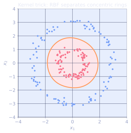
The polynomial-kernel identity matches the explicit feature map, the RBF Gram matrix is PSD, and the kernel SVM separates concentric circles that no linear classifier can split.

Exercises

Exercise 1. For one-dimensional inputs, write the explicit feature map $\phi$ for the kernel $k(x, x') = (xx' + 1)^2$ and confirm $\phi(x)^\top \phi(x') = k(x, x')$.

Exercise 2. Using only the definition $k(x, x') = \phi(x)^\top \phi(x')$, prove that the sum $k(x, x') = k_1(x, x') + k_2(x, x')$ of two valid kernels is itself a valid kernel.

Exercise 3 (code). Confirm the degree-2 identity above on random 2D inputs, then show that $g(x, x') = x^\top x' - 1$ is not a valid kernel by exhibiting a finite set whose Gram matrix has a negative eigenvalue.

import numpy as np

rng = np.random.default_rng(0)
X = rng.normal(size=(6, 2))

def phi(X):
    x1, x2 = X[:, 0], X[:, 1]
    return np.column_stack([np.ones(len(X)), np.sqrt(2) * x1, np.sqrt(2) * x2,
                            x1**2, x2**2, np.sqrt(2) * x1 * x2])

K_direct = (1 + X @ X.T)**2
K_phi = phi(X) @ phi(X).T
assert np.allclose(K_direct, K_phi)           # the kernel identity holds

# g(x, x') = x^T x' - 1 violates the PSD requirement
G = X @ X.T - 1.0
min_eig = np.linalg.eigvalsh(G).min()
print(f"min eigenvalue of g-Gram: {min_eig:.3f}")
assert min_eig < 0                            # not positive semidefinite

The next lesson tours the kernel zoo: RBF, polynomial, and string kernels.

References

- [1]Boser, B. E., Guyon, I. M., & Vapnik, V. N. (1992). "A training algorithm for optimal margin classifiers". COLT. Introduces the kernel trick for maximum-margin classifiers (doi:10.1145/130385.130401).↩
- [2]Schölkopf, B., & Smola, A. J. (2002). Learning with Kernels. MIT Press. The reference treatment of Mercer kernels, RKHS, and kernel construction.↩