Superposition and polysemanticity

Mechanistic interpretability hopes to find one feature per neuron: "neuron 73 detects banana-ness." In practice, individual neurons are polysemantic: they activate for multiple unrelated concepts (curve detectors, sports, capitalized words, ...).

Superposition (Elhage et al., 2022) provides a principled explanation: a network with $d$ neurons can represent more than $d$ features by storing them in nearly-orthogonal directions, accepting small interference costs in exchange for larger representational capacity[1].

The toy model

Consider a network trying to represent $n > d$ sparse features using $d$ dimensions. Feature $i$ has value $f_i \ge 0$, occurring with probability $p$ (sparsity: most features are 0 most of the time).

The model maps features $\mathbf{f} \in \mathbb{R}^n$ to activations $\mathbf{h} = W \mathbf{f}$ (encode) and reconstructs as $\hat{\mathbf{f}} = \text{ReLU}(W^\top \mathbf{h})$ (decode), where $W \in \mathbb{R}^{d \times n}$.

The reconstruction loss (with importance weights $I_i$):

When does superposition occur? Training reveals a phase transition:

• No superposition (features < neurons): each feature gets its own dimension. Zero interference.
• Superposition (features > neurons): features are stored in nearly-orthogonal directions. Each feature has some interference with others, but the benefit of storing more features outweighs the cost when features are sparse.

The critical variable is $1 - S$ where $S$ is sparsity (probability of being nonzero). Dense features (high $1-S$) compete for dimensions; sparse features (low $1-S$) happily share directions because they rarely co-occur.

Implementing the toy model

import numpy as np

def relu(x):
    return np.maximum(0, x)

def train_superposition_model(n_features, n_hidden, sparsity, importance_decay=0.9,
                               n_steps=5000, lr=0.01, seed=0):
    """
    n_features: number of features to represent (> n_hidden for superposition regime)
    n_hidden:   dimension of the hidden layer
    sparsity:   probability that each feature is 0
    """
    rng   = np.random.default_rng(seed)
    W     = rng.normal(0, 0.1, (n_hidden, n_features))
    # Feature importances: I_i = importance_decay^i (most important feature = i=0)
    I     = importance_decay ** np.arange(n_features)
    losses = []

    for step in range(n_steps):
        # Sample sparse feature batch (batch_size=256)
        B = 256
        f = rng.uniform(0, 1, (B, n_features))
        mask = rng.random((B, n_features)) > sparsity   # 1 with prob (1-sparsity)
        f *= mask   # sparse features

        # Forward pass
        h    = f @ W.T              # (B, n_hidden): encode
        f_hat = relu(h @ W)         # (B, n_features): decode

        # Loss
        diff  = f - f_hat
        loss  = (I[None, :] * diff ** 2).mean()

        # Backward (manual gradient for W)
        # dL/d(f_hat) = -2 * I * diff / (B * n_features)
        df_hat = -2 * I[None, :] * diff / (B * n_features)
        # f_hat = relu(h @ W), gradient only where h @ W > 0
        mask_relu = (h @ W) > 0
        df_hat_masked = df_hat * mask_relu
        # dL/dW += h.T @ df_hat_masked (contribution from decode)
        # dL/dW += (df_hat_masked @ W.T).T @ f (contribution from encode, chain rule)
        grad_W  = h.T @ df_hat_masked   # (n_hidden, n_features)
        grad_W += (f.T @ (df_hat_masked @ W.T)).T   # encode contribution

        W -= lr * grad_W
        losses.append(loss)

    return W, losses

# Superposition regime: 10 features in 5 dimensions
W, losses = train_superposition_model(n_features=10, n_hidden=5, sparsity=0.7)
print(f"Final loss: {losses[-1]:.5f}")

# Measure interference: ideally columns of W are nearly orthogonal
col_norms = np.linalg.norm(W, axis=0)
W_norm = W / (col_norms[None, :] + 1e-9)
gram = W_norm.T @ W_norm   # (n_features, n_features)
off_diag = gram - np.eye(gram.shape[0])
print(f"Max off-diagonal Gram entry: {np.abs(off_diag).max():.4f}")
print(f"Mean absolute interference: {np.abs(off_diag).mean():.4f}")
print("(Lower = more orthogonal = better superposition)")

The phase transition

The key prediction of the superposition hypothesis: as sparsity increases (features become rarer), a phase transition occurs from the "no superposition" regime to the "superposition" regime. At the phase boundary, the model abruptly starts encoding more features than it has dimensions.

Implications for interpretability:

• Neurons are not the right unit of analysis (they are polysemantic).
• Features are directions in activation space, not individual neurons.
• Finding features requires decomposing the activation space into interpretable directions (which sparse autoencoders do, as the next lesson shows).

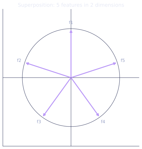
The geometry of superposition

In the superposition regime, features are stored in directions that form a regular polytope structure:

• $n = d + 1$ features fit in $d$ dimensions as vertices of a simplex (all pairwise cosine similarities equal $-1/d$).
• $n = 2d$ features fit as an antipodal pair arrangement.
• More features require denser packings.

This geometric structure predicts which features will "collapse" (merge into one direction) when the network must compress more features into fewer dimensions under limited sparsity.

Exercises

Exercise 1. Suppose $n = d + 1$ features are stored as the vertices of a regular simplex in $d$ dimensions, so all pairwise cosine similarities are equal. Using the fact that the unit vectors sum to zero, derive that the shared cosine similarity is exactly $-\tfrac{1}{d}$, and evaluate it for $d = 4$.

Exercise 2. Two features each fire independently with probability $p$ (so sparsity is $1 - p$ in the lesson's convention of "probability of being zero" $= 1 - p$). They share a single stored direction (collision). Interference costs the model only when both fire at once. Compute the probability of a collision event as a function of $p$, and explain why high sparsity (small $p$) makes sharing a direction nearly free.

Exercise 3 (code). Train the lesson's toy model in both regimes and confirm the qualitative prediction: with more features than dimensions and high sparsity, the model packs features into near-orthogonal directions (small off-diagonal Gram entries), whereas with dense features it cannot, and the off-diagonal interference is larger.

import numpy as np

def relu(x):
    return np.maximum(0, x)

def train(n_features, n_hidden, sparsity, n_steps=4000, lr=0.01, seed=0):
    rng = np.random.default_rng(seed)
    W = rng.normal(0, 0.1, (n_hidden, n_features))
    I = 0.9 ** np.arange(n_features)
    for _ in range(n_steps):
        B = 256
        f = rng.uniform(0, 1, (B, n_features))
        f *= (rng.random((B, n_features)) > sparsity)   # zero with prob = sparsity
        h = f @ W.T
        f_hat = relu(h @ W)
        diff = f - f_hat
        df_hat = -2 * I[None, :] * diff / (B * n_features)
        df_hat *= (h @ W) > 0
        grad_W = h.T @ df_hat + (f.T @ (df_hat @ W.T)).T
        W -= lr * grad_W
    return W

def mean_interference(W):
    norms = np.linalg.norm(W, axis=0)
    Wn = W / (norms[None, :] + 1e-9)
    gram = Wn.T @ Wn
    off = gram - np.eye(gram.shape[0])
    return np.abs(off).mean()

# 10 features, 5 dimensions. Sparse vs dense.
W_sparse = train(n_features=10, n_hidden=5, sparsity=0.9, seed=0)   # rarely co-active
W_dense  = train(n_features=10, n_hidden=5, sparsity=0.1, seed=0)   # usually co-active

intf_sparse = mean_interference(W_sparse)
intf_dense  = mean_interference(W_dense)
print(f"mean |off-diagonal| interference  sparse: {intf_sparse:.4f}")
print(f"mean |off-diagonal| interference  dense:  {intf_dense:.4f}")

# Sparse features pack with less interference than dense ones.
assert intf_sparse < intf_dense

The next lesson takes the practical consequence of superposition seriously: since features are directions rather than neurons, recovering them calls for a dedicated decomposition tool, the sparse autoencoder.

References

- [1]Elhage, N., et al. (2022). "Toy models of superposition". Transformer Circuits Thread. transformer-circuits.pub. Source of the toy model, the phase transition, and the polytope geometry.↩