Probing classifiers

A language model processes text and produces hidden states at each layer. Probing asks: what information is encoded in these representations? Does layer 5 of BERT know the part-of-speech of each token? Does layer 20 of GPT-2 encode whether a sentence is grammatically correct?

Probing answers these questions by training simple classifiers on frozen activations and measuring how accurately they predict linguistic properties.

The probing methodology

Probing protocol:

1. Choose a linguistic property $y$ (POS tag, dependency label, sentence length, subject's grammatical number, sentiment, ...).
2. Collect a labeled dataset $(x_i, y_i)$ where $x_i$ is a sentence and $y_i$ is the property value.
3. Run the language model on each $x_i$ and extract the hidden state $h_i^{(\ell)}$ at layer $\ell$ for the target token (or the [CLS] embedding for sentence-level properties).
4. Train a linear classifier (logistic regression) on the frozen representations: $\hat{y} = W h + b$.
5. Evaluate probe accuracy on held-out data.

A linear probe is standard: if the property is linearly decodable, it is strongly represented in the activation[1]. A nonlinear probe can reveal information present but entangled; the distinction matters for interpretation.

Implementation

import numpy as np
from sklearn.linear_model import LogisticRegression
from sklearn.model_selection import train_test_split
from sklearn.preprocessing import LabelEncoder

def extract_activations(model, sentences, layer_idx, token_idx=0):
    """
    Simulate extracting hidden states at layer `layer_idx` for `token_idx`.
    In practice, use model hooks or HuggingFace's `output_hidden_states=True`.
    Returns: (N, d) array of activations.
    """
    rng = np.random.default_rng(42)
    N, d = len(sentences), 64
    # Simulate: activations loosely correlated with sentence properties
    return rng.normal(0, 1, (N, d))

def probe(activations, labels):
    """Train a linear probe and report accuracy."""
    le = LabelEncoder()
    y  = le.fit_transform(labels)
    X_train, X_test, y_train, y_test = train_test_split(
        activations, y, test_size=0.2, random_state=0
    )
    clf = LogisticRegression(max_iter=1000, C=1.0)
    clf.fit(X_train, y_train)
    acc = clf.score(X_test, y_test)
    return acc, le.classes_

# Simulated data: sentences with POS tags for a target token
sentences = [
    "The cat sat on the mat",
    "A dog runs in the park",
    "She walked quickly to school",
    "He loves reading books daily",
    "The sun rises every morning",
] * 20

# Simulate: target token POS alternates for demo
pos_labels = (["NOUN", "VERB"] * (len(sentences) // 2 + 1))[:len(sentences)]

for layer in [0, 3, 6, 9, 11]:  # BERT-base has 12 layers
    acts = extract_activations(None, sentences, layer)
    acc, classes = probe(acts, pos_labels)
    print(f"Layer {layer:2d}: POS probe accuracy = {acc:.3f}")

Interpreting probe results

High accuracy: the property is encoded linearly in the representation. This is evidence that the model represents the property.

Low accuracy: either the model does not represent the property, or it is encoded nonlinearly. A nonlinear probe (MLP) can disambiguate.

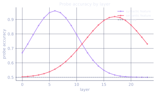
Layer-wise analysis: plotting accuracy across layers reveals how information is processed. In BERT:

• Layer 0-3: surface features (POS, named entities).
• Layer 4-8: syntactic structure (dependency relations, constituency).
• Layer 9-12: semantic content (coreference, semantic roles).

This pattern, discovered by Tenney et al. (2019), suggests the transformer learns the NLP pipeline bottom-up.

Caveats: the probing critique

High probe accuracy does not imply that the model uses the representation. The model might linearly encode POS tags in layer 5 but never use them for downstream tasks. The information is there but may be irrelevant.

Control tasks (Hewitt and Liang, 2019): train a probe on a random label assignment (shuffled labels). If the probe accuracy is high on random labels, the representation has enough capacity to encode anything, so high accuracy on real labels is less meaningful.

Mutual information probing: instead of accuracy, measure how much information (mutual information) the representation carries about the property. More principled but harder to compute.

Causal intervention: to test if the model actually uses a representation, modify it directly (activation patching, next lesson) and observe the effect on output. Probing is correlation; intervention is causation.

Probing for factual knowledge

Beyond linguistic properties, probing tests whether factual knowledge is stored in specific layers. Meng et al. (2022, ROME) found that in GPT-style models:

• Subject token representations (the entity being asked about) store factual associations.
• These associations are stored primarily in FFN layers at middle-to-late depths.
• Editing a specific FFN layer's weights updates the corresponding fact without damaging unrelated facts (within limits).

This finding motivates model editing -- surgically modifying factual representations without full retraining.

Exercises

Exercise 1. A binary linear probe is trained on frozen activations and reaches $92\%$ accuracy. A control probe, trained on the same activations but with the labels randomly shuffled, reaches $78\%$ accuracy. The metric of interest is selectivity, defined as real-task accuracy minus control accuracy. Compute the selectivity, and explain what a small selectivity would have told you even if the real-task accuracy were high.

Exercise 2. Layer-wise probe accuracies for part-of-speech are $0.71, 0.86, 0.90, 0.84, 0.79$ at layers $0, 3, 6, 9, 11$. A colleague concludes "layer 6 is where the model stores POS." State two distinct reasons this conclusion is unjustified, drawing on the probing critique in this lesson.

Exercise 3 (code). Implement a linear probe from scratch in numpy (no sklearn). Build a synthetic dataset where the label is linearly decodable from the activations, fit a probe by least squares, and verify it generalizes on held-out data well above chance. Then verify a control probe on shuffled labels does not.

import numpy as np

rng = np.random.default_rng(0)
N, d = 600, 16

# A ground-truth direction encodes a binary label linearly in the activations.
w_true = rng.normal(0, 1, d)
X = rng.normal(0, 1, (N, d))
score = X @ w_true
y = (score > 0).astype(float)   # balanced binary label (score is mean-zero)

# Split into train / test.
tr, te = slice(0, 500), slice(500, N)

def fit_probe(Xtr, ytr):
    # Ridge least squares on centered targets, w = (X^T X + eps I)^{-1} X^T (y - mean).
    A = Xtr.T @ Xtr + 1e-3 * np.eye(Xtr.shape[1])
    return np.linalg.solve(A, Xtr.T @ (ytr - ytr.mean()))

def accuracy(w, Xte, yte):
    pred = (Xte @ w > 0).astype(float)   # boundary at 0, targets were centered
    return (pred == yte).mean()

# Real probe.
w = fit_probe(X[tr], y[tr])
real_acc = accuracy(w, X[te], y[te])

# Control probe: shuffle the training labels, refit.
y_shuf = rng.permutation(y[tr])
w_ctrl = fit_probe(X[tr], y_shuf)
ctrl_acc = accuracy(w_ctrl, X[te], y[te])

print(f"real probe test accuracy:    {real_acc:.3f}")
print(f"control probe test accuracy: {ctrl_acc:.3f}")
print(f"selectivity:                 {real_acc - ctrl_acc:.3f}")

# The real probe decodes the planted direction; the control cannot generalize.
assert real_acc > 0.85
assert ctrl_acc < 0.65
assert real_acc - ctrl_acc > 0.20

The next lesson moves from correlation to causation: instead of reading activations with a probe, it edits them and watches the output change.

References

- [1]Alain, G., & Bengio, Y. (2017). "Understanding intermediate layers using linear classifier probes". ICLR Workshop. arXiv:1610.01644. Introduces the linear-probe methodology used here.↩