Sparse autoencoders

Superposition tells us that LLM activations store many features as directions in a continuous vector space, with individual neurons being polysemantic. Sparse autoencoders (SAEs) attempt to reverse-engineer this encoding: find a dictionary of interpretable, monosemantic features such that each activation can be reconstructed as a sparse linear combination of dictionary vectors[1, 2].

The idea

Given residual stream activations $\mathbf{x} \in \mathbb{R}^d$ (from a specific layer, token position), find:

• A dictionary $\mathbf{D} \in \mathbb{R}^{d \times m}$ with $m \gg d$ features (columns).
• A sparse code $\mathbf{c} \in \mathbb{R}^m_{\ge 0}$ such that $\mathbf{x} \approx \mathbf{D} \mathbf{c}$.
• Sparse: most entries of $\mathbf{c}$ are zero; only a few features are "on" at any time.

If the features are monosemantic (each column of $\mathbf{D}$ corresponds to a single interpretable concept), this gives a human-readable decomposition of any activation.

The SAE architecture

The SAE is a one-hidden-layer autoencoder with L1 regularization:

where $W_{\text{enc}} \in \mathbb{R}^{m \times d}$, $W_{\text{dec}} \in \mathbb{R}^{d \times m}$, and decoder columns $W_{\text{dec}}[:, i]$ are constrained to unit norm (to prevent the model from hiding large activations in small codes).

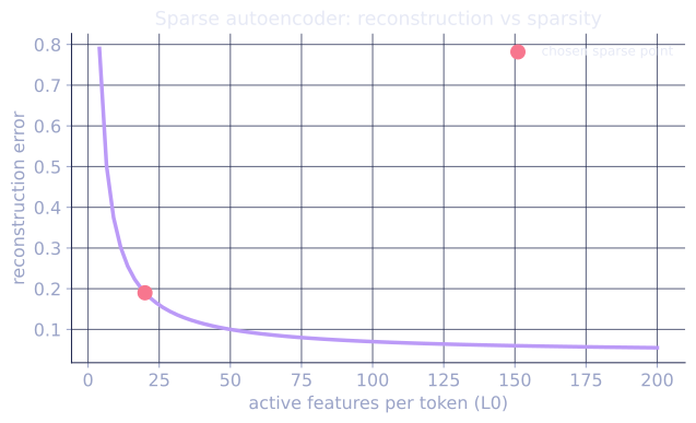
The ReLU ensures $\mathbf{c} \ge 0$. The L1 penalty enforces sparsity: features are zero unless their activation benefit exceeds the penalty.

Training

SAEs are trained on large caches of LLM activations:

1. Run the LLM on a large corpus (e.g., 1B tokens).
2. Cache activations at a specific layer and token position.
3. Train the SAE on these activations with the reconstruction + sparsity loss.

The SAE never touches the LLM's weights -- it is trained entirely on activations. The expansion factor $m/d$ is typically 4-64 (e.g., $d = 768$, $m = 32{,}768$).

Implementation

import numpy as np

class SparseAutoencoder:
    def __init__(self, d, m, lam=0.01, seed=0):
        """d: activation dim, m: dictionary size (m >> d)."""
        rng = np.random.default_rng(seed)
        self.lam = lam
        self.W_enc = rng.normal(0, 0.02, (m, d))
        self.b_enc = np.zeros(m)
        self.W_dec = rng.normal(0, 0.02, (d, m))
        self.b_dec = np.zeros(d)
        # Normalize decoder columns
        self._normalize_dec()

    def _normalize_dec(self):
        norms = np.linalg.norm(self.W_dec, axis=0, keepdims=True) + 1e-9
        self.W_dec /= norms

    def encode(self, x):
        """x: (B, d). Returns sparse codes (B, m)."""
        pre_act = (x - self.b_dec) @ self.W_enc.T + self.b_enc   # (B, m)
        return np.maximum(0, pre_act)   # ReLU -> non-negative codes

    def decode(self, c):
        """c: (B, m). Returns reconstruction (B, d)."""
        return c @ self.W_dec.T + self.b_dec

    def loss(self, x):
        c    = self.encode(x)
        x_hat = self.decode(c)
        recon = np.mean((x - x_hat) ** 2)
        sparse = self.lam * np.mean(np.abs(c))
        return recon + sparse, recon, sparse

    def step(self, x, lr=1e-3):
        """SGD update."""
        B, d = x.shape
        m = self.W_enc.shape[0]
        c    = self.encode(x)
        x_hat = self.decode(c)
        # Gradients
        d_recon = 2 * (x_hat - x) / B          # (B, d)
        dW_dec  = d_recon.T @ c                 # (d, m)
        db_dec  = d_recon.mean(axis=0)          # (d,)
        # Through decode: d_recon flows to code
        dc = d_recon @ self.W_dec               # (B, m)
        # Through encode (ReLU gate)
        gate = (c > 0).astype(float)
        dc_gated = dc * gate                    # (B, m)
        # L1 gradient
        dc_l1 = self.lam * np.sign(c) * gate   # (B, m)
        dc_total = dc_gated + dc_l1
        dW_enc = dc_total.T @ (x - self.b_dec) / B   # (m, d)
        db_enc = dc_total.mean(axis=0)
        # Update
        self.W_enc -= lr * dW_enc
        self.b_enc -= lr * db_enc
        self.W_dec -= lr * dW_dec
        self.b_dec -= lr * db_dec
        self._normalize_dec()

# Train on synthetic activations
d, m = 16, 64
sae = SparseAutoencoder(d, m, lam=0.05)

rng = np.random.default_rng(1)
# Simulate sparse ground-truth features (5 of 16 active at once)
for step in range(2000):
    x = rng.normal(0, 1, (256, d))
    sae.step(x, lr=5e-4)

total_loss, recon, sparse = sae.loss(rng.normal(0, 1, (1000, d)))
c = sae.encode(rng.normal(0, 1, (1000, d)))
print(f"Reconstruction loss: {recon:.5f}")
print(f"Sparsity (L1):       {sparse:.5f}")
print(f"Mean active features per token: {(c > 0).sum(axis=1).mean():.1f} / {m}")

Evaluating SAE features

Feature interpretation: for each dictionary feature $i$ (column of $W_{\text{dec}}$), find the top-activating tokens across the corpus and read off the pattern. Monosemantic features consistently activate for one concept (e.g., "the word 'Toronto'", "all-caps text", "code comments").

Ablation: zero out feature $i$ ($c_i \leftarrow 0$) and observe the change in the model's output. If ablating a "France-related" feature suppresses the logit of "Paris" and "French", the feature causally influences the model's behavior.

F1 / Jaccard: compare the SAE's active features on a text to human-annotated semantic categories.

Large-scale SAE results

Anthropic trained SAEs on Claude 3 Sonnet's residual stream (Templeton et al., 2024)[3]:

• Extracted ~34 million features.
• Features included: cities, emotions, programming concepts, biographical facts.
• Found a "banana" feature, a "slavery" feature, a "1996" feature, a "sycophancy" feature.
• Ablating a "hatred of races" feature reduced racist outputs without hurting general capability.

This is the closest the field has come to a full dictionary of neural network concepts. The remaining challenge: coverage is incomplete (many activations are not explained by identified features), and higher-order interactions between features remain opaque.

Exercises

Exercise 1. An SAE has dictionary size $m = 32{,}768$ and on a given token its code $\mathbf{c}$ has exactly $20$ nonzero entries. The activation dimension is $d = 768$. Compute the L0 sparsity (number of active features) and the corresponding fraction of the dictionary that is active. Then explain why the L1 penalty $\lambda\|\mathbf{c}\|_1$, rather than a direct L0 count, is what the training loss uses.

Exercise 2. A decoder column $W_{\text{dec}}[:, i]$ is constrained to unit norm. Show that without this constraint, the L1 penalty can be driven arbitrarily small without changing the reconstruction, making the sparsity term meaningless. (Hint: consider scaling column $i$ by a constant $s$ and the code entry $c_i$ by $1/s$.)

Exercise 3 (code). Generate synthetic activations that are a sparse non-negative combination of a known overcomplete dictionary, then train the SparseAutoencoder from this lesson on them. Verify that after training the reconstruction error is small and the learned codes are sparser (fewer active features per token) than at initialization.

import numpy as np

# Reuse the lesson's SAE.
class SparseAutoencoder:
    def __init__(self, d, m, lam=0.01, seed=0):
        rng = np.random.default_rng(seed)
        self.lam = lam
        self.W_enc = rng.normal(0, 0.02, (m, d))
        self.b_enc = np.zeros(m)
        self.W_dec = rng.normal(0, 0.02, (d, m))
        self.b_dec = np.zeros(d)
        self._normalize_dec()

    def _normalize_dec(self):
        norms = np.linalg.norm(self.W_dec, axis=0, keepdims=True) + 1e-9
        self.W_dec /= norms

    def encode(self, x):
        return np.maximum(0, (x - self.b_dec) @ self.W_enc.T + self.b_enc)

    def decode(self, c):
        return c @ self.W_dec.T + self.b_dec

    def step(self, x, lr=1e-3):
        B = x.shape[0]
        c = self.encode(x)
        x_hat = self.decode(c)
        d_recon = 2 * (x_hat - x) / B
        dW_dec = d_recon.T @ c
        db_dec = d_recon.mean(axis=0)
        dc = d_recon @ self.W_dec
        gate = (c > 0).astype(float)
        dc_total = dc * gate + self.lam * np.sign(c) * gate
        dW_enc = dc_total.T @ (x - self.b_dec) / B
        db_enc = dc_total.mean(axis=0)
        self.W_enc -= lr * dW_enc
        self.b_enc -= lr * db_enc
        self.W_dec -= lr * dW_dec
        self.b_dec -= lr * db_dec
        self._normalize_dec()

rng = np.random.default_rng(2)
d, m_true = 16, 40
D_true = rng.normal(0, 1, (d, m_true))           # ground-truth overcomplete dictionary
D_true /= np.linalg.norm(D_true, axis=0, keepdims=True)

def sample_activations(B):
    # Each sample fires ~4 of 40 latent features, non-negative.
    codes = np.zeros((B, m_true))
    for b in range(B):
        on = rng.choice(m_true, size=4, replace=False)
        codes[b, on] = rng.uniform(0.5, 2.0, size=4)
    return codes @ D_true.T

sae = SparseAutoencoder(d, m=64, lam=0.02, seed=0)

x0 = sample_activations(1000)
init_active = (sae.encode(x0) > 0).sum(axis=1).mean()
init_err = np.mean((x0 - sae.decode(sae.encode(x0))) ** 2)

for _ in range(4000):
    sae.step(sample_activations(256), lr=1e-3)

xt = sample_activations(1000)
final_active = (sae.encode(xt) > 0).sum(axis=1).mean()
final_err = np.mean((xt - sae.decode(sae.encode(xt))) ** 2)

print(f"reconstruction MSE: init {init_err:.4f} -> final {final_err:.4f}")
print(f"active features/token: init {init_active:.1f} -> final {final_active:.1f}")

# Training lowers reconstruction error and concentrates activity into fewer features.
assert final_err < init_err
assert final_active < init_active
assert final_err < 0.5

The next lesson puts these features to work for control: steering the model by adding a feature's direction back into the residual stream at inference time.

References

- [1]Bricken, T., et al. (2023). "Towards monosemanticity: decomposing language models with dictionary learning". Transformer Circuits Thread. transformer-circuits.pub. The SAE dictionary-learning recipe.↩
- [2]Cunningham, H., Ewart, A., Riggs, L., Huben, R., & Sharkey, L. (2023). "Sparse autoencoders find highly interpretable features in language models". arXiv:2309.08600. Concurrent evidence that SAE features are interpretable.↩
- [3]Templeton, A., et al. (2024). "Scaling monosemanticity: extracting interpretable features from Claude 3 Sonnet". Transformer Circuits Thread. transformer-circuits.pub. The frontier-scale results quoted here.↩