One-class SVM

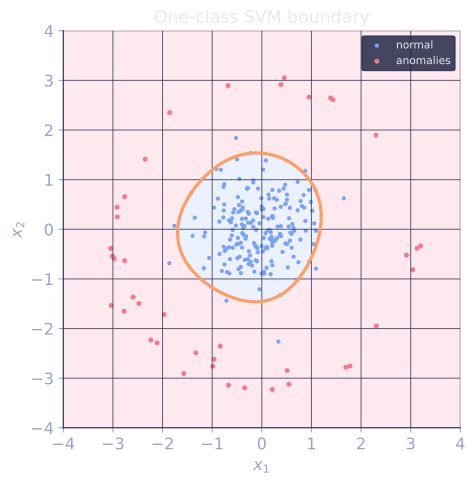
The two-class SVM finds the hyperplane separating two labeled classes. The one-class SVM treats anomaly detection as a degenerate classification: all the training data is "normal", and the algorithm finds the smallest region in feature space that contains the bulk of it. Anything outside is flagged as anomalous[2].

Two equivalent formulations

Two algorithms are commonly called "one-class SVM" and they are equivalent under a change of kernel:

Schölkopf's $\nu$-SVM. Find a hyperplane in kernel feature space that separates the data from the origin with maximum margin[1]. Equivalently, solve

The hyperparameter $\nu \in (0, 1]$ is both an upper bound on the fraction of training points outside the boundary (i.e. flagged) and a lower bound on the fraction of support vectors.

Tax & Duin's SVDD (Support Vector Data Description). Find the smallest ball in feature space containing the data:

With the RBF kernel, the two are equivalent: every point in feature space has the same norm $k(x, x) = 1$, so the smallest enclosing ball and the hyperplane farthest from the origin are the same boundary.

The decision function

After training, score a query point by

Flag $x$ as anomalous if $f(x) < 0$, normal if $f(x) > 0$. The magnitude of $f$ is a continuous score, useful for ranking.

Hyperparameters

• $\nu$: the fraction of allowed outliers. Set to your expected anomaly rate. Smaller $\nu$ = stricter boundary (fewer flags), larger $\nu$ = looser.
• RBF $\gamma$: bandwidth. Small $\gamma$ produces wide, smooth boundaries (under-fits the normal region); large $\gamma$ produces tight boundaries (over-fits, flags everything). Cross-validate against expected anomaly rate or held-out anomalies if available.

Strengths

• Kernel flexibility: any positive-definite kernel works, so the boundary can be arbitrarily nonlinear.
• Sparse representation: only support vectors matter at test time.
• Provable bound on training-error rate via $\nu$.

Limits

• Cost: training a kernel SVM is $O(n^2)$ memory and worse in time. Impractical above ~10^5 samples.
• High dimensions: like all distance-based methods, suffers from the curse.
• Hyperparameter sensitivity: $\gamma$ and $\nu$ both need cross-validation, and the boundary is sensitive to both.

For large datasets, Isolation Forest (previous lesson) or deep AD methods (next lesson) are usually faster.

Check it on arrays

import numpy as np

rng = np.random.default_rng(0)

# Normal cluster + ring of anomalies far away
n_normal = 200
X_normal = rng.normal(scale=0.7, size=(n_normal, 2))
theta = np.linspace(0, 2 * np.pi, 30, endpoint=False)
X_anom = 4 * np.column_stack([np.cos(theta), np.sin(theta)]) + 0.1 * rng.normal(size=(30, 2))

# One-class SVM via projected gradient on the dual:
# max -0.5 alpha^T K alpha + sum(alpha)   s.t. 0 <= alpha <= 1/(nu n),  sum(alpha) = 1
def rbf(X1, X2, gamma):
    d2 = np.sum(X1**2, 1)[:, None] + np.sum(X2**2, 1) - 2 * X1 @ X2.T
    return np.exp(-gamma * d2)

def one_class_svm(X, nu=0.1, gamma=0.5, steps=5000, lr=1e-3):
    n = len(X)
    K = rbf(X, X, gamma)
    alpha = np.full(n, 1 / n)                            # init to feasible
    cap = 1.0 / (nu * n)
    for _ in range(steps):
        grad = np.ones(n) - K @ alpha
        alpha = np.clip(alpha + lr * grad, 0, cap)
        alpha /= alpha.sum()                              # project onto sum = 1
        alpha = np.clip(alpha, 0, cap)
    # rho recovered from support vectors at the boundary (0 < alpha < cap)
    boundary = (alpha > 1e-4) & (alpha < cap - 1e-4)
    rho = np.median((K @ alpha)[boundary]) if boundary.any() else np.median(K @ alpha)
    return alpha, rho, gamma

alpha, rho, gamma = one_class_svm(X_normal, nu=0.05, gamma=0.5)

def score(X_query, X_train, alpha, rho, gamma):
    return rbf(X_query, X_train, gamma) @ alpha - rho

scores_normal = score(X_normal, X_normal, alpha, rho, gamma)
scores_anom = score(X_anom, X_normal, alpha, rho, gamma)
print(f"mean score on normal:    {scores_normal.mean():.3f}  (>= 0 = normal)")
print(f"mean score on anomalies: {scores_anom.mean():.3f}")
print(f"fraction of anomalies flagged: {(scores_anom < 0).mean():.2f}")
print(f"fraction of normal points flagged: {(scores_normal < 0).mean():.2f}  (nu = 0.05 budget)")

The one-class SVM keeps normal points on the positive side of the boundary and flags most of the ring anomalies; the false-positive rate on normal points sits near the $\nu$ budget.

Exercises

Exercise 1. The decision function is $f(x) = \sum_{i \in SV}\alpha_i\, k(x_i, x) - \rho$. Suppose a model has two support vectors with weights $\alpha_1 = 0.6$, $\alpha_2 = 0.4$ and offset $\rho = 0.5$, using an RBF kernel $k(x_i, x) = e^{-\gamma\lVert x_i - x\rVert^2}$ with $\gamma = 1$. A query point sits at squared distance $0.25$ from the first support vector and $4$ from the second. Compute $f(x)$ and classify the point.

Exercise 2. In Schölkopf's $\nu$-SVM, $\nu \in (0, 1]$ is both an upper bound on the fraction of training points that end up outside the boundary and a lower bound on the fraction of support vectors. Explain why these two bounds force a floor on how few support vectors the model can use, and what that implies for the test-time cost when $\nu$ is large.

Exercise 3 (code). Implement the uniform-weight special case of the one-class SVM, where every training point gets equal weight $\alpha_i = 1/n$ so the score is $f(x) = \frac{1}{n}\sum_i k(x_i, x) - \rho$. Set $\rho$ to the $\nu$-quantile of the training scores. On the lesson's normal cluster plus ring of anomalies, check that every ring point is flagged and the normal false-positive rate matches $\nu$.

import numpy as np

rng = np.random.default_rng(0)

# Uniform-weight one-class scorer: every training point has weight 1/n, so
# f(x) = mean_i k(x_i, x) - rho is large near the dense normal region and
# small far from it. A stable special case of the one-class SVM.
def rbf(X1, X2, gamma):
    d2 = np.sum(X1**2, 1)[:, None] + np.sum(X2**2, 1) - 2 * X1 @ X2.T
    return np.exp(-gamma * np.maximum(d2, 0.0))

n_normal = 200
X_normal = rng.normal(scale=0.7, size=(n_normal, 2))
theta = np.linspace(0, 2 * np.pi, 30, endpoint=False)
X_anom = 4 * np.column_stack([np.cos(theta), np.sin(theta)]) + 0.1 * rng.normal(size=(30, 2))

gamma = 0.5
alpha = np.full(n_normal, 1.0 / n_normal)            # uniform weights

nu = 0.05
train_sim = rbf(X_normal, X_normal, gamma) @ alpha
rho = np.quantile(train_sim, nu)                     # nu-quantile offset

def f(Xq):
    return rbf(Xq, X_normal, gamma) @ alpha - rho

s_normal = f(X_normal)
s_anom = f(X_anom)
print(f"mean score on normal:    {s_normal.mean():.3f}")
print(f"mean score on anomalies: {s_anom.mean():.3f}")
print(f"fraction of anomalies flagged: {(s_anom < 0).mean():.2f}")
print(f"fraction of normal flagged:    {(s_normal < 0).mean():.2f}  (nu = {nu})")

assert (s_anom < 0).all()                            # every ring point flagged
assert abs((s_normal < 0).mean() - nu) < 0.02        # normal false-positive rate ~ nu

The next lesson uses neural-network reconstruction error as the AD signal.

References

- [1]Schölkopf, B., Platt, J. C., Shawe-Taylor, J., Smola, A. J., & Williamson, R. C. (2001). "Estimating the support of a high-dimensional distribution". Neural Computation, 13(7), 1443-1471. doi:10.1162/089976601750264965. Introduces the -SVM that separates data from the origin and the bound on outliers and support vectors.↩
- [2]Chandola, V., Banerjee, A., & Kumar, V. (2009). "Anomaly detection: a survey". ACM Computing Surveys, 41(3), 1-58. doi:10.1145/1541880.1541882. Frames one-class SVMs within classification-based anomaly detection.↩