Isolation Forest

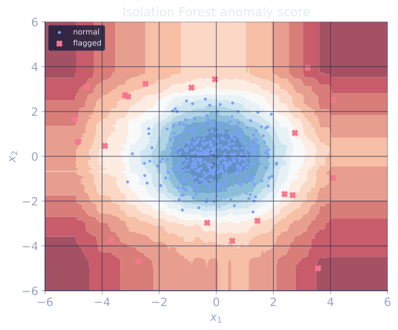
Density-based and distance-based AD struggle in high dimensions. Isolation Forest flips the problem on its head: instead of building a model of the normal data and measuring deviation, it directly measures how easy each point is to isolate with random splits. Anomalies, being few and different, get isolated in shorter paths than normal points[1].

The idea

Build a forest of isolation trees on random subsamples. Each tree recursively splits the data on a random feature at a random threshold until each point is isolated in its own leaf.

The path length to isolate point $x$ is the number of splits required. Anomalies, being far from the mass of the data, tend to be isolated after few splits (they are easy to peel off). Normal points need many splits (they live in dense regions where any split keeps neighbors together).

The anomaly score combines path lengths across trees and normalizes:

where $E[h(x)]$ is the mean path length across trees and $c(n)$ is the expected path length of an unsuccessful search in a binary tree of $n$ points (a normalization constant). Scores close to 1 indicate anomalies; scores below 0.5 indicate normal points.

Algorithm

For each tree:

1. Subsample $\psi$ points (typical $\psi = 256$).
2. Repeat: pick a random feature, pick a random threshold uniformly within the current node's range, split. Stop at unit-size leaves or at a max depth $\lceil\log_2 \psi\rceil$.

For a query $x$, compute its path length in each tree (depth at which it lands in a leaf) and average across the forest.

Why subsample to $\psi = 256$

Two reasons:

• Computational: each tree is $O(\psi \log \psi)$, so the whole forest is small regardless of $n$.
• Statistical: with a large training set, normal points crowd anomalies and obscure their isolation. A small subsample lets each anomaly stand out against fewer normal neighbors.

Pleasantly counterintuitive: smaller subsamples often make anomaly detection better, not worse.

Strengths

• Scales linearly in dataset size (after the small subsample).
• No distance metric: works in mixed-type tabular data.
• High-dimensional friendly: random feature selection means each tree sees a different subset of features.
• Out-of-the-box useful: usually works with default parameters, which is why surveys list it among the standard tabular AD baselines[2].

Limits

• Random splits do not use the data's geometry, so subtle anomalies in rotated subspaces can be missed.
• Pure-categorical features without ordering are awkward (no natural threshold).
• Score interpretation requires the normalization constant; raw path lengths are not directly comparable across $\psi$.

Check it on arrays

import numpy as np

rng = np.random.default_rng(0)

# Normal data + a few anomalies in 3D
n_normal, n_anom = 500, 15
X_normal = rng.normal(loc=[0, 0, 0], scale=[1, 1, 1], size=(n_normal, 3))
X_anom = rng.uniform(low=-6, high=6, size=(n_anom, 3))
X = np.vstack([X_normal, X_anom])
true_anom = np.concatenate([np.zeros(n_normal), np.ones(n_anom)])

def random_isolation_tree(X, rng, max_depth):
    if len(X) <= 1 or max_depth == 0:
        return ("leaf", len(X))
    d = X.shape[1]
    j = rng.integers(d)
    lo, hi = X[:, j].min(), X[:, j].max()
    if hi == lo:
        return ("leaf", len(X))
    t = rng.uniform(lo, hi)
    mask = X[:, j] < t
    if mask.sum() == 0 or (~mask).sum() == 0:
        return ("leaf", len(X))
    return ("node", j, t,
            random_isolation_tree(X[mask], rng, max_depth - 1),
            random_isolation_tree(X[~mask], rng, max_depth - 1))

def path_length(tree, x, depth=0):
    if tree[0] == "leaf":
        n = tree[1]
        if n <= 1: return depth
        # add expected path length adjustment for the remaining n points
        c = 2 * (np.log(n - 1) + 0.5772156649) - 2 * (n - 1) / n
        return depth + c
    _, j, t, left, right = tree
    if x[j] < t:
        return path_length(left, x, depth + 1)
    return path_length(right, x, depth + 1)

def isolation_forest(X, n_trees=100, psi=256, rng=rng):
    max_depth = int(np.ceil(np.log2(max(psi, 2))))
    trees = []
    for _ in range(n_trees):
        sample = X[rng.choice(len(X), size=min(psi, len(X)), replace=False)]
        trees.append(random_isolation_tree(sample, rng, max_depth))
    return trees, psi

def anomaly_score(trees, psi, X):
    n = len(X)
    paths = np.zeros(n)
    for t in trees:
        for i, x in enumerate(X):
            paths[i] += path_length(t, x)
    paths /= len(trees)
    c_psi = 2 * (np.log(psi - 1) + 0.5772156649) - 2 * (psi - 1) / psi
    return 2 ** (-paths / c_psi)

trees, psi = isolation_forest(X, n_trees=50, psi=128)
scores = anomaly_score(trees, psi, X)

# Higher score = more anomalous; pick top 20 as anomalies
top_idx = np.argsort(scores)[-20:]
n_correct = int(true_anom[top_idx].sum())
print(f"top-20 score-ranked points: {n_correct}/{n_anom} true anomalies recovered")
print(f"mean score on normal: {scores[true_anom == 0].mean():.3f}")
print(f"mean score on anomalies: {scores[true_anom == 1].mean():.3f}")

Isolation Forest ranks most of the planted anomalies in the top 20 by score, with a clear gap between normal and anomalous mean scores.

Exercises

Exercise 1. A point lands in a leaf at depth $4$ in one tree and depth $6$ in another, with both leaves holding a single point. Using $s(x) = 2^{-E[h(x)]/c(n)}$ with a subsample of $n = 256$ (so $c(256) \approx 10.24$), compute the anomaly score and say whether it reads as anomalous or normal.

Exercise 2. The normalization $c(n) = 2H_{n-1} - 2(n-1)/n$, where $H_{n-1} = \sum_{i=1}^{n-1} 1/i$ is the harmonic number, is the expected path length of an unsuccessful search in a binary search tree of $n$ points. Show that $c(n)$ is strictly increasing in $n$, and explain why dividing $E[h(x)]$ by $c(n)$ is what makes scores comparable across different subsample sizes $\psi$.

Exercise 3 (code). Build isolation trees on a 1D sample of $256$ standard normal points. Score one far outlier at $x = 12$ and one typical point at $x = 0$ by averaging path lengths over $200$ trees. Confirm the outlier has the shorter mean path and the higher anomaly score.

import numpy as np

# c(n): expected unsuccessful-search path length in a binary tree of n points.
def c(n):
    if n <= 1:
        return 0.0
    return 2 * (np.log(n - 1) + 0.5772156649) - 2 * (n - 1) / n

rng = np.random.default_rng(0)

def build_tree(X, rng, max_depth):
    if len(X) <= 1 or max_depth == 0:
        return ("leaf", len(X))
    j = rng.integers(X.shape[1])
    lo, hi = X[:, j].min(), X[:, j].max()
    if hi == lo:
        return ("leaf", len(X))
    t = rng.uniform(lo, hi)
    mask = X[:, j] < t
    if mask.sum() == 0 or (~mask).sum() == 0:
        return ("leaf", len(X))
    return ("node", j, t,
            build_tree(X[mask], rng, max_depth - 1),
            build_tree(X[~mask], rng, max_depth - 1))

def path_length(tree, x, depth=0):
    if tree[0] == "leaf":
        return depth + c(tree[1])
    _, j, t, left, right = tree
    return path_length(left if x[j] < t else right, x, depth + 1)

X = rng.normal(size=(256, 1))
x_outlier = np.array([12.0])
x_typical = np.array([0.0])

n_trees = 200
max_depth = int(np.ceil(np.log2(256)))
h_out, h_typ = 0.0, 0.0
for _ in range(n_trees):
    tree = build_tree(X, rng, max_depth)
    h_out += path_length(tree, x_outlier)
    h_typ += path_length(tree, x_typical)
h_out /= n_trees; h_typ /= n_trees

cpsi = c(256)
s_out = 2 ** (-h_out / cpsi)
s_typ = 2 ** (-h_typ / cpsi)
print(f"mean path length: outlier={h_out:.3f}, typical={h_typ:.3f}")
print(f"anomaly score:    outlier={s_out:.3f}, typical={s_typ:.3f}")

assert h_out < h_typ          # the far point is isolated faster
assert s_out > s_typ          # so it scores as more anomalous

The next lesson takes a completely different geometric view: enclose the normal region with a kernel SVM.

References

- [1]Liu, F. T., Ting, K. M., & Zhou, Z.-H. (2008). "Isolation forest". ICDM. doi:10.1109/ICDM.2008.17. The original isolation-by-path-length algorithm, with the score and the subsample.↩
- [2]Chandola, V., Banerjee, A., & Kumar, V. (2009). "Anomaly detection: a survey". ACM Computing Surveys, 41(3), 1-58. doi:10.1145/1541880.1541882. Positions isolation and tree-based methods among the broader AD taxonomy.↩