Conditioning and numerical stability

A numerical answer can be wrong for two reasons: the problem itself amplifies input perturbations (it is ill-conditioned), or the algorithm introduces excess rounding error (it is unstable). These are independent. A well-conditioned problem solved by an unstable algorithm gives a wrong answer; an ill-conditioned problem solved by the perfect algorithm still gives a wrong answer. Knowing which is which tells you whether to change the algorithm or change the problem.

Conditioning: a property of the problem

The condition number of a problem measures how much the output changes when the input is perturbed. For a function $f(x)$, the relative condition number is

It is the worst-case ratio of relative output change to relative input change[1]. If the input is known to floating-point precision $\varepsilon_{\text{machine}}$, the output is unavoidably uncertain by about $\kappa \cdot \varepsilon_{\text{machine}}$, regardless of how the computation is performed.

The condition number of a linear system

For $Ax = b$ with $A$ invertible, perturbing $b$ by $\Delta b$ perturbs $x$ by $\Delta x = A^{-1}\Delta b$. The condition number of solving the system is

and in the 2-norm equals the ratio of largest to smallest singular value:

Derivation. From $b = Ax$, $\lVert b\rVert \le \lVert A\rVert\,\lVert x\rVert$, so $\lVert x\rVert \ge \lVert b\rVert/\lVert A\rVert$. From $\Delta x = A^{-1}\Delta b$, $\lVert \Delta x\rVert \le \lVert A^{-1}\rVert\,\lVert\Delta b\rVert$. Dividing,

identifying $\kappa(A)$ as the amplification factor. $\qquad\blacksquare$

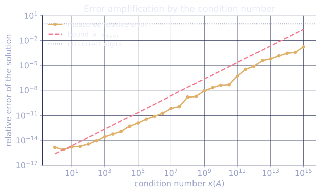
A matrix with $\kappa = 10^{12}$ loses 12 digits of precision: even the perfect solver, with double-precision input, returns only 4 correct digits.

Stability: a property of the algorithm

An algorithm is backward stable if the computed answer is the exact answer to a slightly perturbed problem: $\hat y = f(x + \Delta x)$ with $\lVert \Delta x\rVert = O(\varepsilon_{\text{machine}})\lVert x\rVert$[2]. Backward stability is the strongest practical guarantee, because combined with conditioning it yields the forward error bound

The total error is the product of problem conditioning and algorithm stability. A stable algorithm cannot improve a bad condition number; an unstable algorithm contaminates even a perfectly conditioned problem.

Two routes for least squares

The normal equations $A^\top A x = A^\top b$ have condition number $\kappa(A^\top A) = \kappa(A)^2$: squaring the conditioning of the original problem. The QR or SVD routes (from the A1 least-squares lesson) keep the conditioning at $\kappa(A)$ rather than $\kappa(A)^2$[3]. Both routes solve the same problem; their stability differs.

Check it on arrays

import numpy as np

rng = np.random.default_rng(0)
eps = np.finfo(float).eps

# Build a matrix with controlled condition number via the SVD.
def make_A(n, kappa):
    U = np.linalg.qr(rng.normal(size=(n, n)))[0]
    V = np.linalg.qr(rng.normal(size=(n, n)))[0]
    s = np.geomspace(1.0, 1.0 / kappa, n)
    return U @ np.diag(s) @ V.T

n = 50
for kappa in [1e2, 1e6, 1e12]:
    A = make_A(n, kappa)
    x_true = rng.normal(size=n)
    b = A @ x_true
    x_hat = np.linalg.solve(A, b)
    err = np.linalg.norm(x_hat - x_true) / np.linalg.norm(x_true)
    bound = kappa * eps
    print(f"kappa={kappa:>.0e}: rel error {err:.2e}, bound kappa*eps {bound:.2e}")

# Squaring the conditioning: solve via normal equations vs QR
A = make_A(n, 1e6)
b = A @ rng.normal(size=n)
x_normal = np.linalg.solve(A.T @ A, A.T @ b)             # uses kappa^2
Q, R = np.linalg.qr(A); x_qr = np.linalg.solve(R, Q.T @ b)  # uses kappa
truth = np.linalg.solve(A, b)
print("normal-eq error:", np.linalg.norm(x_normal - truth))
print("QR-route error: ", np.linalg.norm(x_qr - truth))

The relative error grows with the condition number as predicted, and the normal- equations route loses precision the QR route preserves.

Exercises

Exercise 1. A matrix $A$ has $\sigma_{\max} = 10$ and $\sigma_{\min} = 10^{-5}$. Compute $\kappa_2(A)$, and state how many correct digits a backward-stable solver of $Ax = b$ returns when the input is given to double precision ($\varepsilon_{\text{machine}} \approx 2.2 \times 10^{-16}$).

Exercise 2. Show that for the normal equations $A^\top A x = A^\top b$, the condition number satisfies $\kappa_2(A^\top A) = \kappa_2(A)^2$. Use the SVD $A = U \Sigma V^\top$.

Exercise 3 (code). Build a matrix with controlled $\kappa_2 = 10^8$ via its SVD, solve $Ax = b$ for a known $x$, and confirm the relative error stays under the bound $\kappa_2 \cdot \varepsilon_{\text{machine}}$.

import numpy as np

rng = np.random.default_rng(0)
eps = np.finfo(float).eps
n, kappa = 40, 1e8

# Controlled condition number: singular values geomspaced from 1 to 1/kappa.
U = np.linalg.qr(rng.normal(size=(n, n)))[0]
V = np.linalg.qr(rng.normal(size=(n, n)))[0]
s = np.geomspace(1.0, 1.0 / kappa, n)
A = U @ np.diag(s) @ V.T

assert np.isclose(np.linalg.cond(A), kappa, rtol=1e-3)

x_true = rng.normal(size=n)
b = A @ x_true
x_hat = np.linalg.solve(A, b)
rel_err = np.linalg.norm(x_hat - x_true) / np.linalg.norm(x_true)

assert rel_err <= kappa * eps          # forward-error bound holds
print("rel error:", rel_err, "  bound kappa*eps:", kappa * eps)

The next lesson zooms in on the most common source of stability loss: subtracting near-equal numbers.

References

- [1]Trefethen, L. N., & Bau, D. (1997). Numerical Linear Algebra. SIAM. Conditioning, stability, and the condition number (Lectures 12-15).↩
- [2]Higham, N. J. (2002). Accuracy and Stability of Numerical Algorithms (2nd ed.). SIAM. The definitive treatment of backward stability and forward error (doi:10.1137/1.9780898718027).↩
- [3]Golub, G. H., & Van Loan, C. F. (2013). Matrix Computations (4th ed.). Johns Hopkins University Press. Normal equations versus QR for least squares.↩