Fixed-point and iterative methods

Many problems have no closed-form solution, but can be rewritten as $x = T(x)$ for some map $T$. Iterative methods start from a guess and apply $T$ repeatedly until the sequence settles. The condition that makes this work, $T$ being a contraction, also gives an explicit error bound and convergence rate, which is the template used in everything from linear solvers to optimization to MCMC[1].

Fixed points

A fixed point of a map $T: \mathbb{R}^n \to \mathbb{R}^n$ is a point $x^\star$ with $T(x^\star) = x^\star$. The fixed-point iteration is the simple loop

If the sequence converges, its limit is a fixed point: $\lim x_{k+1} = \lim T(x_k) = T(\lim x_k)$ when $T$ is continuous. The question is when the sequence converges and how fast.

Contraction mappings

$T$ is a contraction with constant $L < 1$ if it brings every pair of points strictly closer together:

Banach fixed-point theorem. A contraction on a complete space has a unique fixed point $x^\star$, and from any $x_0$ the iteration converges to it at a geometric rate:

Proof sketch. Apply the contraction property iteratively: $\lVert x_{k+1} - x_k\rVert \le L\lVert x_k - x_{k-1}\rVert \le L^k \lVert x_1 - x_0\rVert$. The geometric series $\sum_k L^k$ converges since $L < 1$, so $\{x_k\}$ is Cauchy and has a limit $x^\star$. Continuity of $T$ shows $x^\star$ is a fixed point. Uniqueness: two fixed points $x, y$ would give $\lVert x - y\rVert = \lVert T(x) - T(y)\rVert \le L\lVert x - y\rVert$, forcing $\lVert x - y\rVert = 0$. $\qquad\blacksquare$

The rate $L^k$ is linear convergence: each step shrinks the error by a constant factor. Reaching accuracy $\varepsilon$ takes $O(\log(1/\varepsilon)/\log(1/L))$ steps.

The constant $L$ is the whole story, and its scale is worth feeling. To reach $\varepsilon = 10^{-6}$:

• $L = 0.5$ (error halves each step) needs about 20 steps; after 10 steps the error is already down to $0.5^{10} \approx 10^{-3}$.
• $L = 0.9$ needs about 131 steps; 10 steps only knock the error down to $0.9^{10} \approx 0.35$.
• $L = 0.99$ needs about 1375 steps; 10 steps barely move it, to $0.9^{10}$'s far worse cousin $0.99^{10} \approx 0.90$.

The cosine map below has $L = |T'(x^\star)| = \sin(x^\star) \approx 0.674$, so it sits near the fast end and settles in a few dozen steps.

Newton's method as a fixed-point iteration

Solving $f(x) = 0$ can be cast as the fixed-point iteration $x_{k+1} = T(x_k)$ with $T(x) = x - f(x)/f'(x)$, which is exactly Newton's method. At a simple root, $T'(x^\star) = 1 - (f'(x^\star)^2 - f(x^\star)f''(x^\star))/f'(x^\star)^2 = 0$, so $T$ is more than a contraction near the root: it has zero local derivative, which is the algebraic source of Newton's quadratic convergence.

Jacobi iteration for linear systems

For $Ax = b$ with $A = D + R$ ($D$ the diagonal, $R$ the rest), the Jacobi iteration is

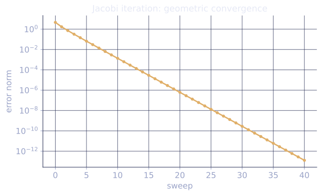
a fixed-point form of the linear system. The iteration matrix is $-D^{-1}R$, and the iteration converges if the spectral radius (the largest eigenvalue magnitude) is less than 1, which holds for strictly diagonally dominant $A$ ($|a_{ii}| > \sum_{j \neq i}|a_{ij}|$). Jacobi and its variant Gauss-Seidel are the original iterative linear solvers, the predecessors of conjugate gradient[2, 3].

Check it on arrays

import numpy as np

# 1) Fixed-point iteration for cos: x = cos(x), Dottie number ~0.7390851...
T = np.cos
x = 0.0
errs = []
for _ in range(60):
    errs.append(x)
    x = T(x)
print("Dottie fixed point:", round(x, 8))
print("|T'(x*)| =", round(abs(-np.sin(x)), 4), "  < 1 (contraction near x*)")

# 2) Jacobi for a diagonally dominant linear system
rng = np.random.default_rng(0)
n = 30
A = rng.normal(size=(n, n))
np.fill_diagonal(A, np.abs(A).sum(axis=1) + 1.0)         # make strictly diag. dominant
b = rng.normal(size=n)

D = np.diag(np.diag(A)); R = A - D
Dinv = np.diag(1.0 / np.diag(A))
x = np.zeros(n)
gaps = []
truth = np.linalg.solve(A, b)
for _ in range(200):
    x = Dinv @ (b - R @ x)
    gaps.append(np.linalg.norm(x - truth))
# Geometric decay: ratio of consecutive errors should be roughly constant
ratios = np.array(gaps[1:]) / np.array(gaps[:-1])
print(f"Jacobi avg contraction factor: {np.mean(ratios[50:100]):.4f}")
print(f"final error: {gaps[-1]:.2e}")

The cosine iteration settles on the Dottie number with $|T'| < 1$ confirming contraction, and Jacobi converges linearly on the diagonally dominant system.

Exercises

Exercise 1. A contraction has constant $L = 0.8$. Using the geometric bound $\lVert x_k - x^\star\rVert \le L^k \lVert x_0 - x^\star\rVert$, find the smallest $k$ that guarantees the error has dropped below $10^{-3}$ of the initial error.

Exercise 2. Newton's method for $f(x) = x^2 - a$ gives the iteration $x_{k+1} = \tfrac12\left(x_k + \tfrac{a}{x_k}\right)$. Show this is the fixed-point map $T(x) = x - f(x)/f'(x)$, and verify $T'(x^\star) = 0$ at the root $x^\star = \sqrt{a}$.

Exercise 3 (code). Implement Jacobi iteration for a strictly diagonally dominant $Ax = b$ and confirm the error decays geometrically with a contraction factor below $1$ equal to the spectral radius of $-D^{-1}R$.

import numpy as np

rng = np.random.default_rng(0)
n = 20
A = rng.normal(size=(n, n))
np.fill_diagonal(A, np.abs(A).sum(axis=1) + 1.0)   # strictly diagonally dominant
b = rng.normal(size=n)

D = np.diag(np.diag(A))
R = A - D
Dinv = np.diag(1.0 / np.diag(A))
iter_matrix = -Dinv @ R
rho = np.max(np.abs(np.linalg.eigvals(iter_matrix)))   # spectral radius
assert rho < 1.0                                        # convergence condition

truth = np.linalg.solve(A, b)
x = np.zeros(n)
errs = []
for _ in range(40):
    x = Dinv @ (b - R @ x)
    errs.append(np.linalg.norm(x - truth))
errs = np.array(errs)

# Error ratio in the geometric regime (before it hits the rounding floor)
# tracks the spectral radius.
ratios = errs[6:15] / errs[5:14]
assert abs(np.mean(ratios) - rho) < 0.05
print("spectral radius:", round(rho, 4), "  measured ratio:", round(float(np.mean(ratios)), 4))

The next lesson specializes the iterative idea to symmetric positive-definite systems: conjugate gradient.

References

- [1]Trefethen, L. N., & Bau, D. (1997). Numerical Linear Algebra. SIAM. Iteration and convergence of stationary methods (Lectures 27-28).↩
- [2]Saad, Y. (2003). Iterative Methods for Sparse Linear Systems (2nd ed.). SIAM. Jacobi, Gauss-Seidel, and spectral-radius convergence (doi:10.1137/1.9780898718003).↩
- [3]Golub, G. H., & Van Loan, C. F. (2013). Matrix Computations (4th ed.). Johns Hopkins University Press. Classical stationary iterative methods.↩