The conjugate gradient method

For a large symmetric positive-definite system $Ax = b$, direct factorization costs $O(n^3)$ and stores a dense factor. Conjugate gradient (CG) solves it iteratively using only matrix-vector products, finishing in at most $n$ steps in exact arithmetic and far fewer in practice[1]. It is the workhorse for sparse SPD systems and the template for Krylov methods.

CG as minimizing a quadratic

For SPD $A$, solving $Ax = b$ is equivalent to minimizing the quadratic

whose gradient is $\nabla \phi = Ax - b$ (zero exactly at the solution). CG generates iterates $x_0, x_1, \dots$ each of which is the exact minimizer of $\phi$ over a growing Krylov subspace, using only the gradients (residuals) $r_k = b - A x_k$.

$A$-conjugate directions

Two directions $p$ and $q$ are conjugate with respect to $A$ if $p^\top A q = 0$, the $A$-inner-product orthogonality. CG builds an $A$-conjugate set of search directions: each $p_k$ is $A$-orthogonal to all previous ones.

The payoff: minimizing $\phi$ along $A$-conjugate directions one at a time is the same as minimizing it over their span. There is no need to revisit a previous direction once you have stepped along it. After $k$ steps, $x_k$ is the exact minimizer in the $k$-dimensional subspace spanned by the first $k$ directions.

The CG update

Starting from $x_0$ with $r_0 = b - A x_0$ and $p_0 = r_0$, each step does:

1. Step length along the current direction $p_k$ that minimizes $\phi$: $$\alpha_k = \frac{r_k^\top r_k}{p_k^\top A p_k}.$$
2. Update $x_{k+1} = x_k + \alpha_k p_k$ and $r_{k+1} = r_k - \alpha_k A p_k$.
3. New direction $A$-conjugate to all previous: $$\beta_k = \frac{r_{k+1}^\top r_{k+1}}{r_k^\top r_k}, \qquad p_{k+1} = r_{k+1} + \beta_k p_k.$$

The cost per iteration is one matrix-vector product $A p_k$ and a handful of vector operations: $O(n)$ memory plus the cost of multiplying by $A$, which for sparse $A$ scales with the number of nonzeros.

Krylov subspaces and finite termination

The space spanned by $\{r_0, A r_0, A^2 r_0, \dots, A^{k-1} r_0\}$ is the Krylov subspace $\mathcal{K}_k$. CG's $x_k$ minimizes $\phi$ over $x_0 + \mathcal{K}_k$. In exact arithmetic, the dimension of the Krylov subspace grows by one each step until it contains the true solution, so CG terminates in at most $n$ steps with $x_n = x^\star$[2].

Convergence rate

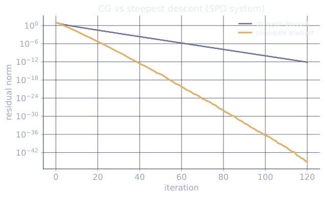
In practice CG converges much faster than $n$ when the eigenvalues of $A$ cluster. With condition number $\kappa = \lambda_{\max}/\lambda_{\min}$, the error satisfies

a rate of $\sqrt\kappa$ like Nesterov's acceleration. Preconditioning (solving $M^{-1}A x = M^{-1}b$ for a cheap $M \approx A$) shrinks the effective condition number and is what makes CG practical for ill-conditioned systems[3].

Check it on arrays

import numpy as np

rng = np.random.default_rng(0)

# Random SPD system of moderate condition number.
n = 200
B = rng.normal(size=(n, n))
A = B @ B.T + 0.5 * np.eye(n)                              # SPD
b = rng.normal(size=n)

def cg(A, b, tol=1e-10, max_iter=None):
    x = np.zeros_like(b)
    r = b - A @ x
    p = r.copy()
    rs_old = r @ r
    history = []
    for k in range(max_iter or len(b) + 5):
        Ap = A @ p
        alpha = rs_old / (p @ Ap)
        x = x + alpha * p
        r = r - alpha * Ap
        rs_new = r @ r
        history.append(np.sqrt(rs_new))
        if rs_new < tol**2:
            break
        beta = rs_new / rs_old
        p = r + beta * p
        rs_old = rs_new
    return x, history

x_cg, hist = cg(A, b)
x_true = np.linalg.solve(A, b)
print(f"CG converged in {len(hist)} iterations")
print(f"final residual: {hist[-1]:.2e}")
print(f"error vs direct solve: {np.linalg.norm(x_cg - x_true):.2e}")
print(f"finite-termination bound: <= n = {n}")

CG reaches the solution in fewer iterations than the dimension when the spectrum is favorable, with residual decaying geometrically.

Exercises

Exercise 1. For the SPD system with $A = \left(\begin{smallmatrix} 4 & 1 \\ 1 & 3 \end{smallmatrix}\right)$, $b = (1, 2)^\top$, and $x_0 = 0$, compute the first CG step length $\alpha_0$ and the iterate $x_1$ by hand.

Exercise 2. With condition number $\kappa = 4$, evaluate the CG error-reduction factor $\frac{\sqrt\kappa - 1}{\sqrt\kappa + 1}$ per step, and find how many steps drive the $A$-norm error below $10^{-6}$ of its start (ignore the leading factor of $2$).

Exercise 3 (code). Implement CG for a random SPD system and verify two properties: the residuals $r_k$ are mutually orthogonal, and the solution matches a direct solve.

import numpy as np

rng = np.random.default_rng(0)
n = 40
# Well-conditioned SPD matrix: eigenvalues spread evenly in [1, 10].
Q = np.linalg.qr(rng.normal(size=(n, n)))[0]
A = Q @ np.diag(np.linspace(1.0, 10.0, n)) @ Q.T
b = rng.normal(size=n)

x = np.zeros(n)
r = b - A @ x
p = r.copy()
rs_old = r @ r
residual_vecs = [r.copy()]
for _ in range(n):
    Ap = A @ p
    alpha = rs_old / (p @ Ap)
    x = x + alpha * p
    r = r - alpha * Ap
    rs_new = r @ r
    residual_vecs.append(r.copy())
    if rs_new < 1e-20:
        break
    p = r + (rs_new / rs_old) * p
    rs_old = rs_new

# Residuals are mutually orthogonal (a defining CG property). Check the early
# iterates, before the residuals shrink to the rounding floor.
R = np.array(residual_vecs[:10])
R = R / np.linalg.norm(R, axis=1, keepdims=True)     # unit-normalize each
G = R @ R.T
off_diag = G - np.diag(np.diag(G))
assert np.max(np.abs(off_diag)) < 1e-8

x_true = np.linalg.solve(A, b)
assert np.linalg.norm(x - x_true) < 1e-6
print("max off-diagonal residual inner product:", np.max(np.abs(off_diag)))

The next lesson generalizes Krylov solvers to nonsymmetric systems with GMRES.

References

- [1]Hestenes, M. R., & Stiefel, E. (1952). "Methods of conjugate gradients for solving linear systems". Journal of Research of the National Bureau of Standards, 49(6), 409-436. The original conjugate-gradient algorithm.↩
- [2]Trefethen, L. N., & Bau, D. (1997). Numerical Linear Algebra. SIAM. CG, Krylov subspaces, and finite termination (Lectures 38-40).↩
- [3]Saad, Y. (2003). Iterative Methods for Sparse Linear Systems (2nd ed.). SIAM. Preconditioned CG and the convergence bound (doi:10.1137/1.9780898718003).↩