Quantization: GPTQ, AWQ, and GGUF

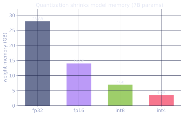
A 70B parameter model at fp16 requires $70 \times 10^9 \times 2 = 140$GB of GPU memory just for weights -- beyond a single GPU. Quantization reduces weight precision from 16-bit floating-point to 8-bit or 4-bit integers, cutting memory by 2-4x at the cost of a small accuracy loss.

Quantization basics

Uniform quantization maps a range $[x_{\min}, x_{\max}]$ to $2^b$ integer levels for bit-width $b$:

$$x_q = \text{round}\!\left(\frac{x - x_{\min}}{x_{\max} - x_{\min}} \cdot (2^b - 1)\right), \quad x_{\text{deq}} = x_q \cdot \frac{x_{\max} - x_{\min}}{2^b - 1} + x_{\min}.$$

Quantization error: $|x - x_{\text{deq}}| \le \Delta/2$ where $\Delta = (x_{\max} - x_{\min}) / (2^b - 1)$.

Per-tensor vs per-channel: computing the scale $\Delta$ per output channel (each row of a weight matrix has its own scale) significantly reduces error compared to a single global scale.

Post-training quantization (PTQ): quantize a pretrained model without retraining. Faster and cheaper than quantization-aware training (QAT), with modest accuracy loss at 4-bit. A key finding at scale is that large activation outliers concentrate in a few feature dimensions, so isolating them lets 8-bit inference match fp16 accuracy[2].

GPTQ: one-shot PTQ for LLMs

GPTQ (Frantar et al., 2022) quantizes weights one layer at a time using second-order information (the Hessian of the layer's output error)[1].

The core algorithm

For a linear layer $Y = WX$ with pretrained weights $W$ and calibration activations $X$:

1. Compute the Hessian of the reconstruction error with respect to $W$: $H = 2 X X^\top$.

2. Quantize columns of $W$ sequentially (Optimal Brain Compression order). For each column $q$ being quantized:

   • Round $W_{:,q}$ to the nearest quantization level.
   • Compensate the remaining unquantized columns for the rounding error: $W_{:,p} \leftarrow W_{:,p} - \frac{[H^{-1}]_{pq}}{[H^{-1}]_{qq}} \cdot \delta_q$, where $\delta_q = W_{:,q} - \text{quant}(W_{:,q})$.

This OBQ (Optimal Brain Quantization) step propagates the quantization error of each column to all remaining columns, minimizing the total output error.

In practice: GPTQ adds block-wise quantization (process 128 columns at a time), lazy batch updates, and Cholesky decomposition for numerical stability. A 175B model quantizes in ~4 hours on a single GPU.

Result: 4-bit GPTQ models lose 1-3 perplexity points on standard benchmarks compared to fp16, with 4x memory reduction.

AWQ: activation-aware weight quantization

AWQ (Lin et al., 2023) observes that not all weights are equally important: quantization error is amplified by large activations. Specifically, if an activation $x_j$ is large, the error in weight $W_{:,j}$ contributes $x_j \cdot \delta W_{:,j}$ to the output error -- large activations make the corresponding weight columns critical.

AWQ algorithm

1. Compute per-channel activation magnitude: $s_j = \mathbb{E}[|x_j|]$ from calibration data.
2. Scale important weight channels (large $s_j$) by a factor $s > 1$ before quantization, and divide the corresponding activations by $s$ to compensate: $W_{:,j}^{\text{scaled}} = W_{:,j} \cdot s_j^{\alpha}$, then absorb $s_j^\alpha$ into the activations (or the previous layer's output).
3. Quantize the scaled weights. The scaling effectively protects important channels from quantization error.

AWQ finds the optimal $\alpha$ per-channel via grid search on calibration data.

AWQ typically outperforms GPTQ at the same bit-width, especially for instruction-tuned models where certain output neurons are highly sensitive to specific input features.

GGUF: portable quantization for CPU/GPU inference

GGUF (formerly GGML, updated format by llama.cpp) is a file format and quantization scheme designed for inference on consumer hardware (CPU, Apple Silicon, small NVIDIA GPUs).

Key design choices:

• Mixed-precision: different layers can have different bit-widths. Embedding and output layers (which have the most parameters and are most sensitive) are kept at higher precision than FFN layers.
• Block quantization: weights are quantized in blocks of 32 or 64 with a per-block scale factor, balancing accuracy and overhead.
• CPU-optimized: uses AVX2/AVX-512 SIMD instructions for fast integer matrix multiplication on x86; NEON on ARM.

GGUF quantization levels (for llama.cpp):

• Q8_0: 8-bit, near-lossless.
• Q5_K_M: 5-bit, good quality-size balance.
• Q4_K_M: 4-bit, recommended for most consumer hardware.
• Q3_K_M: 3-bit, aggressive compression.
• Q2_K: 2-bit, significant quality loss.

Memory comparison (70B model)

Format	Bits/weight	Memory
fp16	16	140 GB
int8 (GPTQ)	8	70 GB
int4 (AWQ/GPTQ)	4	35 GB
Q4_K_M (GGUF)	~4.5	~40 GB
Q2_K (GGUF)	~2.6	~25 GB

At Q4_K_M, a 70B model fits on a 2x A40 (48GB each) or a Mac Studio with 192GB unified memory.

Quantization vs. LoRA vs. smaller models

Quantization, LoRA, and using a smaller model are all ways to fit a capable model on limited hardware. The right choice depends on the tradeoff:

• Quantization: best accuracy at low memory cost; no fine-tuning required.
• LoRA + quantization (QLoRA): enables fine-tuning a large model on consumer hardware.
• Smaller model: lower accuracy ceiling; better latency on the same hardware.

Exercises

Exercise 1. A weight column has values in the range $[x_{\min}, x_{\max}] = [-0.4, 0.6]$. Using uniform quantization, compute the step size $\Delta$ at 4-bit and at 8-bit precision, and the worst-case quantization error $\Delta/2$ for each.

Solution

Step 1. The range spans $x_{\max} - x_{\min} = 0.6 - (-0.4) = 1.0$. The step is $\Delta = (x_{\max} - x_{\min}) / (2^b - 1)$.

Step 2. At $b = 4$, there are $2^4 - 1 = 15$ intervals:

$$\Delta_4 = \frac{1.0}{15} = 0.0667, \qquad \Delta_4/2 = 0.0333.$$

Step 3. At $b = 8$, there are $2^8 - 1 = 255$ intervals:

$$\Delta_8 = \frac{1.0}{255} = 0.00392, \qquad \Delta_8/2 = 0.00196.$$

Each extra bit halves the step size, so going from 4-bit to 8-bit shrinks the worst-case error by a factor $255/15 = 17$, close to the $2^4 = 16$ expected from the four added bits (the small excess is the $2^b - 1$ versus $2^b$ correction).

Exercise 2. Estimate the on-disk size of a 13B-parameter model at fp16, int8, and int4, ignoring per-channel scale overhead. Then explain why a real Q4_K_M GGUF file of the same model is closer to $\approx 7.5$ GB than to the $6.5$ GB a pure 4-bit count predicts.

Solution

Step 1. Bytes per weight are bits over 8: fp16 is $2$ bytes, int8 is $1$ byte, int4 is $0.5$ bytes. Multiply by $13 \times 10^9$ parameters:

$$\text{fp16} = 26 \text{ GB}, \quad \text{int8} = 13 \text{ GB}, \quad \text{int4} = 6.5 \text{ GB}.$$

Step 2. Q4_K_M is not uniformly 4-bit. Block quantization attaches a scale (and often a min) per block of 32 or 64 weights, which adds overhead, and the most sensitive tensors (embeddings, output projection, some attention layers) are kept at 5 or 6 bits. The mixed precision and per-block metadata push the effective rate to roughly $4.5$ bits per weight, so $13 \times 10^9 \times 4.5 / 8 \approx 7.3$ GB, matching the observed $\approx 7.5$ GB rather than the flat $6.5$ GB.

Exercise 3. A team must serve a 70B model on a single 80 GB A100 with room for roughly 30 GB of KV cache at their target batch size, leaving about 50 GB for weights. They consider int8 GPTQ ($70$ GB), int4 AWQ ($35$ GB), and a 34B fp16 model ($68$ GB). Which fit, and what is the central tradeoff between the two viable LLM options?

Solution

Step 1. Compare each weight footprint against the $50$ GB budget: int8 GPTQ at $70$ GB does not fit; the 34B fp16 model at $68$ GB does not fit; int4 AWQ at $35$ GB fits with $15$ GB to spare.

Step 2. Only int4 AWQ of the 70B fits on this single GPU. The realistic alternatives are then int4-quantize the 70B (this option) or step down to a smaller model that fits at higher precision. The tradeoff is capability versus precision: the quantized 70B keeps the larger model's knowledge and reasoning ceiling at the cost of a 1-3 perplexity-point degradation from 4-bit rounding, while a smaller fp16 model avoids quantization error but has a lower accuracy ceiling. For most tasks the quantized larger model wins, which is why int4 serving of large models is the common production choice.

---

References

1. [1]Frantar, E., Ashkboos, S., Hoefler, T., & Alistarh, D. (2023). "GPTQ: accurate post-training quantization for generative pre-trained transformers". ICLR. arXiv:2210.17323. One-shot Hessian-based weight quantization to 3-4 bits.↩
2. [2]Dettmers, T., Lewis, M., Belkada, Y., & Zettlemoyer, L. (2022). "LLM.int8(): 8-bit matrix multiplication for transformers at scale". NeurIPS. arXiv:2208.07339. Mixed int8/fp16 decomposition that isolates emergent activation outliers.↩