 AI Knowledge Tree
KV cache
Cache key and value tensors for all previous tokens so each new token incurs only one new attention row, reducing per-token cost from O(T^2) to O(T).
Without caching, generating a response of tokens requires forward passes, each attending over an increasingly long sequence. The -th forward pass computes attention over all tokens: total cost .
The KV cache eliminates this redundancy: compute and store the key and value matrices for all previous tokens, then reuse them for each new token[1].
Why keys and values are reusable
At each attention layer, for position (a previously generated token):
The token does not change after it is generated. Neither does the weight matrix or . Therefore and are identical in every forward pass that includes position . There is no need to recompute them.
Queries are different: the query at position is , which is computed fresh at each step (it depends on the new token ).
The cached forward pass
Prefill phase: process the full prompt in one forward pass (all tokens in parallel), compute all K and V tensors, store them in the cache.
Decode phase: for each new token:
- Compute for the new token only.
- Append to the cache.
- Compute attention: attends over the full cache (all for ).
- Produce logits for token .
Each decode step costs (one attention row), not .
Memory cost of the KV cache
For a model with layers, attention heads, head dimension , and a sequence of tokens at precision bf16 (2 bytes):
The factor of 2 is for keys and values. For LLaMA-3 70B (, , , using GQA):
At tokens: GB per request. At tokens: GB.
This is why long-context serving is memory-bottlenecked. Techniques like PagedAttention (next-to-next lesson) manage this memory efficiently.
Prefill vs decode throughput
The two phases have different hardware characteristics:
| Phase | Compute bound? | Bottleneck |
|---|---|---|
| Prefill | Yes (large matrix multiply) | GPU compute |
| Decode | No (sequential, small QK multiply) | Memory bandwidth |
During decode, the GPU spends most time loading the model weights and KV cache from HBM (high-bandwidth memory) into registers -- not computing. This is why decode throughput is memory-bandwidth limited.
Implementation sketch
import numpy as np

class AttentionWithKVCache:
    def __init__(self, d_model, n_heads, max_len):
        self.h  = n_heads
        self.dk = d_model // n_heads
        self.max_len = max_len
        rng = np.random.default_rng(0)
        s   = 0.02
        self.Wq = rng.normal(0, s, (d_model, d_model))
        self.Wk = rng.normal(0, s, (d_model, d_model))
        self.Wv = rng.normal(0, s, (d_model, d_model))
        self.Wo = rng.normal(0, s, (d_model, d_model))
        d = d_model
        # Pre-allocate KV cache
        self.k_cache = np.zeros((max_len, d))
        self.v_cache = np.zeros((max_len, d))
        self.cache_len = 0

    def prefill(self, x):
        """x: (T, d_model) -- process prompt all at once."""
        T = x.shape[0]
        self.k_cache[:T] = x @ self.Wk
        self.v_cache[:T] = x @ self.Wv
        self.cache_len = T
        # Full attention over prompt
        return self._attend_full(x @ self.Wq, x @ self.Wk, x @ self.Wv)

    def decode_one(self, x_new):
        """x_new: (1, d_model) -- process single new token."""
        k_new = x_new @ self.Wk   # (1, d)
        v_new = x_new @ self.Wv
        # Append to cache
        t = self.cache_len
        self.k_cache[t] = k_new[0]
        self.v_cache[t] = v_new[0]
        self.cache_len += 1
        # Attend: one query row over the full cache
        q = x_new @ self.Wq   # (1, d)
        K = self.k_cache[:self.cache_len]   # (t+1, d)
        V = self.v_cache[:self.cache_len]
        scores = q @ K.T / np.sqrt(self.dk)
        attn   = np.exp(scores - scores.max())
        attn  /= attn.sum()
        return (attn @ V) @ self.Wo   # (1, d)

    def _attend_full(self, Q, K, V):
        T  = Q.shape[0]
        scores = Q @ K.T / np.sqrt(self.dk)
        mask   = np.triu(np.ones((T, T), dtype=bool), k=1)
        scores[mask] = -1e9
        attn = np.exp(scores - scores.max(-1, keepdims=True))
        attn /= attn.sum(-1, keepdims=True)
        return (attn @ V) @ self.Wo

d, h, T_max = 32, 4, 128
attn_layer = AttentionWithKVCache(d, h, T_max)

# Prefill with 5-token prompt
prompt = np.random.randn(5, d)
out_prefill = attn_layer.prefill(prompt)
print("Prefill output shape:", out_prefill.shape)

# Decode 3 more tokens
for i in range(3):
    new_token = np.random.randn(1, d)
    out = attn_layer.decode_one(new_token)
    print(f"  Decode step {i+1}: cache_len={attn_layer.cache_len}, out_norm={np.linalg.norm(out):.3f}")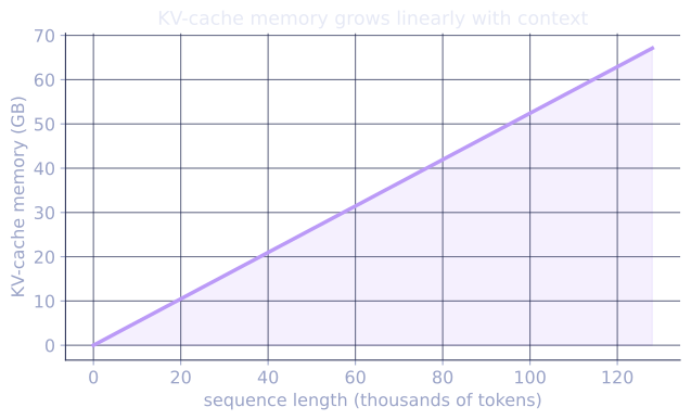
KV cache with GQA
With Grouped-Query Attention (GQA), only key/value heads are stored instead of query heads. The KV cache memory is reduced by -- the primary motivation for GQA in production models[2].
Exercises
Exercise 1. A model has layers, attention heads, head dimension , and stores the KV cache in bf16 (2 bytes), without GQA. Compute the KV cache size, in bytes per token, then in gigabytes for a sequence of tokens.
Solution
Step 1. The per-token size is bytes, where the leading counts keys and values and the trailing is bytes per bf16 number:
Step 2. For tokens, multiply by :
A single 8K-token request already costs GiB of KV cache at full multi-head attention, which is why the cache, not the weights, often caps the batch size.
Exercise 2. Take the model of Exercise 1 and switch to GQA with key/value heads (the 32 query heads share them in groups of 4). By what factor does the KV cache shrink, and what is the new per-token size?
Solution
Step 1. Only the key/value head count changes, from to , so the cache shrinks by .
Step 2. The new per-token size replaces with :
one quarter of the MiB from Exercise 1. GQA trades a small amount of model quality for a smaller cache, which directly raises the achievable batch size and context length.
Exercise 3 (code). Show that the cached decode path computes the same attention output as a from-scratch full-attention pass over the whole sequence. Build a tiny attention layer in numpy, prefill a prompt, decode one token with the cache, and assert the cached output matches recomputing attention over all tokens at once.
Solution
import numpy as np

rng = np.random.default_rng(0)
d = 16
Wk = rng.normal(0, 0.1, (d, d))
Wv = rng.normal(0, 0.1, (d, d))
Wq = rng.normal(0, 0.1, (d, d))

def attend(q, K, V):
    scores = q @ K.T / np.sqrt(d)
    a = np.exp(scores - scores.max(-1, keepdims=True))
    a /= a.sum(-1, keepdims=True)
    return a @ V

X = rng.normal(0, 1, (5, d))          # 4-token prompt + 1 new token
prompt, new = X[:4], X[4:5]

# Cached path: K,V for the prompt are reused, only the new token is appended.
K_cache = prompt @ Wk
V_cache = prompt @ Wv
k_new, v_new = new @ Wk, new @ Wv
K_full = np.vstack([K_cache, k_new])
V_full = np.vstack([V_cache, v_new])
out_cached = attend(new @ Wq, K_full, V_full)

# Recompute from scratch over all 5 tokens, take the last query row.
out_scratch = attend(X @ Wq, X @ Wk, X @ Wv)[4:5]

assert np.allclose(out_cached, out_scratch, atol=1e-12)
print("max abs diff:", np.abs(out_cached - out_scratch).max())
The cached output equals the full recomputation to floating-point precision: reusing the prompt's keys and values changes the cost, not the result.
The next lesson uses one target-model pass to verify several draft tokens at once, turning the memory-bound decode step into a near-parallel one.
References
- [1]Pope, R., et al. (2023). "Efficiently scaling transformer inference". MLSys. arXiv:2211.05102. Analyzes KV-cache memory traffic and the memory-bandwidth limit of the decode phase.↩
- [2]Shazeer, N. (2019). "Fast transformer decoding: one write-head is all you need". arXiv:1911.02150. Multi-query attention shares one K/V head to shrink the cache; GQA generalizes it.↩