Scaling laws: Kaplan and Chinchilla

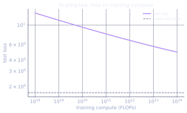
Scaling a language model -- making it larger, training it longer -- predictably improves performance. Scaling laws quantify this relationship as empirical power laws, allowing practitioners to forecast model quality before committing to an expensive training run.

Kaplan et al. (2020): OpenAI scaling laws

Kaplan et al. trained hundreds of models varying three quantities[1]:

• $N$: number of non-embedding parameters.
• $D$: number of training tokens.
• $C$: training compute (FLOPs), approximately $C \approx 6ND$.

Finding 1: power-law relationship between loss and each variable (holding the others constant and large enough):

$$L(N) \approx \left(\frac{N_c}{N}\right)^{\alpha_N}, \quad \alpha_N \approx 0.076,$$ $$L(D) \approx \left(\frac{D_c}{D}\right)^{\alpha_D}, \quad \alpha_D \approx 0.095,$$

where $N_c$ and $D_c$ are fitted constants. Cross-entropy loss on the test set decreases smoothly and predictably as a power law in either $N$ or $D$.

Finding 2: for a fixed compute budget $C$, model size should dominate. Kaplan et al. found that for a given $C$, you should use the largest model that can be trained in the given compute budget (even if it means training for fewer tokens). This led to GPT-3 (175B parameters, 300B tokens) and the trend of training large models for relatively few tokens[2].

Chinchilla (Hoffmann et al., 2022)

Kaplan et al.'s recommendation turned out to be wrong. Hoffmann et al. ran a more careful analysis with better-controlled experiments and found a different optimal allocation[3].

IsoFLOP analysis: for a fixed compute budget $C$, vary $N$ and set $D = C / (6N)$ accordingly. Find the $(N, D)$ that minimizes final loss.

Finding: the optimal allocation satisfies:

$$N^* \propto C^{0.50}, \quad D^* \propto C^{0.50},$$

i.e., model size and token count should scale equally. Doubling compute should be split equally between doubling $N$ and doubling $D$.

The Chinchilla rule of thumb: for a compute-optimal run, train on approximately $D \approx 20 \cdot N$ tokens. For a 70B parameter model: $20 \times 70\text{B} = 1.4\text{T}$ tokens.

Run the $C \approx 6ND$ FLOP count on real models to calibrate what these budgets cost:

• GPT-3 ($N = 175\text{B}$, $D = 300\text{B}$): $C = 6 \times 175\text{B} \times 300\text{B} \approx 3.1 \times 10^{23}$ FLOPs.
• Chinchilla ($N = 70\text{B}$, $D = 1.4\text{T}$): $C \approx 5.9 \times 10^{23}$ FLOPs. Fewer parameters than GPT-3, more compute, and a lower final loss, the result that overturned the Kaplan allocation.
• LLaMA-3 70B ($N = 70\text{B}$, $D = 15\text{T}$): $C \approx 6.3 \times 10^{24}$ FLOPs, about $11\times$ the compute of the Chinchilla-optimal 70B run that reaches a similar loss.

The GPT-3 vs Chinchilla pair is the lesson in one comparison: at roughly the same compute budget, moving parameters into tokens ($175\text{B}/300\text{B}$ to $70\text{B}/1.4\text{T}$) lowered the loss. The LLaMA-3 figure is the deliberate overshoot below.

Chinchilla-optimal models

Model	$N$	$D$ (tokens)	$D/N$
GPT-3	175B	300B	1.7x (undertrained)
Chinchilla	70B	1.4T	20x (optimal)
LLaMA-2 70B	70B	2T	28x (overtrained)
LLaMA-3 70B	70B	15T	214x (heavily overtrained)

LLaMA-2 and LLaMA-3 are deliberately overtrained: the compute budget is allocated toward more tokens at the cost of suboptimal compute efficiency. The reason: inference is expensive in deployment. A smaller, overtrained model is cheaper to serve than a larger, compute-optimal model with the same final loss.

"Compute-optimal" is optimal only for a one-shot training run. If you will run the model for millions of inferences, the optimal allocation shifts: train smaller models longer.

Emergent abilities and phase transitions

A separate empirical finding: certain capabilities (multi-step arithmetic, code generation, multi-hop reasoning) appear abruptly at certain scale thresholds rather than improving gradually. This is called emergence.

The origin is contested:

• Measurement artifact (Wei et al.): metrics with step functions (right/wrong) show phase transitions; smooth metrics show gradual improvement throughout.
• Genuine phase transition: the model qualitatively changes its algorithm for certain tasks at a threshold parameter count.

The implication for practitioners: do not assume smooth performance scaling for all metrics. Some capabilities may be present-or-absent at given scales.

Scaling laws for fine-tuning and alignment

Scaling laws for pretraining don't directly apply to fine-tuning:

• SFT quality saturates faster with data size than pretraining.
• RLHF reward signal quality matters more than quantity.
• Instruction following improves with model scale, but safety and alignment properties don't follow the same power laws.

The practical lesson: spend most of the compute budget on pretraining (where scaling laws give predictable returns), then fine-tune efficiently with smaller datasets.

Exercises

Exercise 1. Using the Chinchilla rule of thumb $D \approx 20N$ and the FLOP count $C \approx 6ND$, find the compute-optimal token count and total training FLOPs for a $13\text{B}$-parameter model.

Solution

Step 1. Apply the rule of thumb: $D \approx 20N = 20 \times 13\text{B} = 260\text{B}$ tokens.

Step 2. Substitute into $C \approx 6ND$ with $N = 13 \times 10^9$ and $D = 260 \times 10^9$:

$$C \approx 6 \times (13 \times 10^9) \times (260 \times 10^9) = 6 \times 3380 \times 10^{18} = 2.028 \times 10^{22} \text{ FLOPs}.$$

So a compute-optimal $13\text{B}$ model trains on about $260\text{B}$ tokens for roughly $2.0 \times 10^{22}$ FLOPs.

Exercise 2. A team has a fixed compute budget $C = 6 \times 10^{23}$ FLOPs and wants the Chinchilla-optimal allocation. Using $D = 20N$ and $C = 6ND$, solve for $N$ and $D$. Then compare the final loss qualitatively against spending the same budget on a $175\text{B}$ model in the Kaplan style.

Solution

Step 1. Substitute $D = 20N$ into $C = 6ND$: $C = 6N(20N) = 120 N^2$, so

$$N = \sqrt{C / 120} = \sqrt{6 \times 10^{23} / 120} = \sqrt{5 \times 10^{21}} \approx 7.07 \times 10^{10} \approx 71\text{B}.$$

Step 2. Then $D = 20N \approx 20 \times 71\text{B} = 1.42\text{T}$ tokens, the Chinchilla 70B/1.4T point, as expected since $C \approx 5.9 \times 10^{23}$ matches that run.

Step 3. Compare allocations. A $175\text{B}$ model at the same budget has $D = C/(6N) = 6\times10^{23} / (6 \times 175\times10^9) \approx 5.7 \times 10^{11} = 0.57\text{T}$ tokens, only $D/N \approx 3.3\times$, far below the optimal $20\times$. It is undertrained, so its final loss is higher than the $71\text{B}/1.4\text{T}$ allocation. This is the GPT-3 vs Chinchilla result: at fixed compute, moving budget from parameters into tokens lowers the loss.

Exercise 3. "Compute-optimal" minimizes loss for a single training run. Argue when a team should deliberately overtrain (the LLaMA-2/3 choice), and quantify the trade-off using the LLaMA-3 70B figure of $D/N \approx 214$ versus the optimal $20$.

Solution

Step 1. State what compute-optimal ignores. The Chinchilla optimum counts only training FLOPs. It does not count inference, which for a deployed model is paid per request across potentially billions of calls.

Step 2. Reframe the objective. The relevant cost is training plus lifetime inference. A smaller model with the same final loss is cheaper to serve (fewer FLOPs per token at inference), so for a heavily-served model it pays to reach that loss with fewer parameters, even at a worse training-compute efficiency.

Step 3. Quantify. LLaMA-3 70B trains on $D/N \approx 214$ tokens per parameter versus the optimal $20$, about $11\times$ more tokens (and roughly $11\times$ the training compute of the Chinchilla-optimal 70B run reaching a similar loss). The team spends that extra training compute once to keep the parameter count at $70\text{B}$ rather than growing the model, trading a one-time training overspend for a permanently cheaper inference cost. The break-even favors overtraining precisely when expected inference volume is large.

The scaling-laws view sets the model size and token budget; the next stage is turning that pretrained base into an instruction follower through supervised fine-tuning.

---

References

1. [1]Kaplan, J., et al. (2020). "Scaling laws for neural language models". arXiv:2001.08361. The original power-law fits for loss versus parameters, data, and compute.↩
2. [2]Brown, T., et al. (2020). "Language models are few-shot learners (GPT-3)". NeurIPS. arXiv:2005.14165. The 175B-parameter, 300B-token model that followed the Kaplan allocation.↩
3. [3]Hoffmann, J., et al. (2022). "Training compute-optimal large language models (Chinchilla)". NeurIPS. arXiv:2203.15556. The IsoFLOP analysis giving the equal-scaling rule and the 20-tokens-per-parameter heuristic.↩