LoRA, QLoRA, and DoRA

Full fine-tuning updates all parameters of a pretrained model. For a 70B model at fp16, this requires $70 \times 10^9 \times 2 \approx 140$GB of gradient memory alone -- far beyond a single GPU and impractical for most users.

Parameter-efficient fine-tuning (PEFT) methods update only a small subset of parameters while freezing the rest, a practical necessity for the supervised and preference fine-tuning stages[1]. LoRA (Hu et al., 2022) is the dominant method: it injects small, trainable rank-decomposition matrices alongside each frozen weight matrix[2].

LoRA: Low-Rank Adaptation

The core idea

For a pretrained weight matrix $W_0 \in \mathbb{R}^{m \times n}$ (e.g., the query projection in a transformer block), instead of training $W_0$ directly, freeze it and learn an additive low-rank update:

where $B \in \mathbb{R}^{m \times r}$ and $A \in \mathbb{R}^{r \times n}$, with rank $r \ll \min(m, n)$.

The forward pass becomes:

Only $A$ and $B$ are trained; $W_0$ is frozen.

Why low-rank?

The intrinsic dimensionality hypothesis (Aghajanyan et al., 2021): the change in weights during fine-tuning lies in a low-dimensional subspace. Empirically, setting $r$ to just 4-16 recovers most of the full fine-tuning performance.

Parameter count

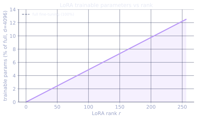
For a weight matrix $W_0 \in \mathbb{R}^{m \times n}$ with LoRA rank $r$:

• LoRA parameters: $r(m + n)$.
• Full fine-tuning parameters: $mn$.
• Reduction: $r(m+n) / mn \approx r/n$ for $m \approx n$.

For a 70B model with $d = 8192$ and $r = 16$:

• Full fine-tuning: all 70B parameters.
• LoRA (on Q, K, V, O projections in all layers): $\approx 16 \times 2 \times 8192 \times 4 \times 80 \approx 84$M parameters ($\sim 0.1\%$ of total).

Initialization

• $A \sim \mathcal{N}(0, \sigma^2)$ (small random).
• $B = 0$.

At initialization, $\Delta W = B A = 0$, so the model starts identically to the pretrained model. This is crucial: the model initially produces the same outputs as before fine-tuning.

Scaling factor

In practice, the update is scaled by $\alpha / r$:

where $\alpha$ is a hyperparameter (often set equal to $r$). This decouples the initialization scale from $r$, making it easier to transfer the same learning rate across different ranks.

Where to apply LoRA

LoRA is applied to the attention weight matrices ($W^Q, W^K, W^V, W^O$) and optionally the FFN matrices. In practice, applying LoRA to all four attention projections gives the best quality-efficiency tradeoff.

Implementation

import numpy as np

class LoRALinear:
    def __init__(self, W0, rank, alpha=1.0, seed=0):
        """W0: pretrained weight (m, n). Frozen."""
        m, n   = W0.shape
        rng    = np.random.default_rng(seed)
        self.W0    = W0
        self.A     = rng.normal(0, 0.02, (rank, n))   # trainable
        self.B     = np.zeros((m, rank))               # trainable, init to 0
        self.scale = alpha / rank

    def forward(self, x):
        """x: (T, n) -> (T, m)"""
        base   = x @ self.W0.T                          # frozen path
        delta  = x @ self.A.T @ self.B.T * self.scale  # adapter path
        return base + delta

# Demo
m, n, r = 64, 32, 4
W0 = np.random.randn(m, n) * 0.02
layer = LoRALinear(W0, rank=r, alpha=r)

x = np.random.randn(10, n)  # 10 tokens, n features
h = layer.forward(x)
print("Output shape:", h.shape)
print("Delta (should be ~0 at init):", np.abs(layer.B @ layer.A).max().round(8))

QLoRA: quantized LoRA

QLoRA (Dettmers et al., 2023) extends LoRA to 4-bit quantized base models:

1. Quantize the base model to 4-bit using NF4 (Normal Float 4), a data type designed to minimize quantization error for normally-distributed weights.
2. Dequantize to bf16 in the forward pass (on-the-fly, per page of 64 weights).
3. Apply LoRA in bf16 on top of the dequantized weights.
4. Backpropagate only through the LoRA adapters.

Result: a 70B model fine-tunable on a single 48GB GPU (A6000), whereas full fine-tuning would require 8+ A100s at bf16.

Double quantization: quantize the quantization constants themselves (the per-block scaling factors) from fp32 to fp8, saving an additional $\sim$0.4 bits per parameter.

DoRA: weight decomposition for LoRA

DoRA (Liu et al., 2024) decomposes the pretrained weight into magnitude and direction, and fine-tunes them separately:

where $m \in \mathbb{R}^{1 \times n}$ is the column-wise norm and $V/\|V\|_c$ is the normalized weight matrix. Fine-tuning uses LoRA for the direction component and a scalar for the magnitude:

DoRA consistently outperforms LoRA at the same rank, approaching full fine-tuning quality at ranks as low as $r = 16$.

Merging LoRA weights

After fine-tuning, merge the adapter into the base model for inference:

No runtime overhead during inference -- the merged weight is identical in shape to $W_0$. Multiple LoRA adapters (for different tasks) can be merged independently or combined with task weights (LoRAHub).

Exercises

Exercise 1. A transformer applies LoRA to all four attention projections ($W^Q, W^K, W^V, W^O$), each of shape $4096 \times 4096$, across 32 layers, with rank $r = 8$. Count the trainable LoRA parameters and compare against full fine-tuning of just those projections.

Exercise 2. At initialization $A \sim \mathcal{N}(0, \sigma^2)$ and $B = 0$, so $\Delta W = BA = 0$ and the model reproduces the pretrained outputs. Show that the gradient of a scalar loss $\ell$ with respect to $A$ is zero at this initialization, while the gradient with respect to $B$ is generally nonzero. Use $\Delta W = BA$ and the chain rule with $G = \partial \ell / \partial \Delta W$.

Exercise 3 (code). Implement the LoRA forward pass with the $\alpha/r$ scaling in numpy and verify two facts: at initialization ($B = 0$) the output equals the frozen base output, and after setting $B$ to a nonzero value the merged weight $W_0 + (\alpha/r) BA$ reproduces the adapted forward pass exactly.

import numpy as np

rng = np.random.default_rng(0)
m, n, r, alpha = 64, 32, 4, 8.0
W0 = rng.normal(0, 0.02, (m, n))
A  = rng.normal(0, 0.02, (r, n))     # trainable
B  = np.zeros((m, r))                # init to 0
scale = alpha / r

x = rng.normal(0, 1, (10, n))        # 10 tokens

def forward(x, W0, A, B, scale):
    base  = x @ W0.T
    delta = (x @ A.T @ B.T) * scale
    return base + delta

# At init B = 0 -> output equals the frozen base path.
out_init = forward(x, W0, A, B, scale)
assert np.allclose(out_init, x @ W0.T)

# After training B becomes nonzero; the merged weight matches the adapter forward.
B = rng.normal(0, 0.1, (m, r))
W_merged = W0 + scale * (B @ A)
assert np.allclose(forward(x, W0, A, B, scale), x @ W_merged.T)
print("merged-weight max abs error:",
      np.abs(forward(x, W0, A, B, scale) - x @ W_merged.T).max())

After fine-tuning, the adapter folds into the base weights and the model is ready to serve; the next lessons turn from parameter-efficiency to the preference signal that fine-tuning optimizes, starting with reward modeling.

References

- [1]Ouyang, L., et al. (2022). "Training language models to follow instructions with human feedback (InstructGPT)". NeurIPS. arXiv:2203.02155. The supervised and preference fine-tuning stages LoRA makes parameter-efficient.↩
- [2]Hu, E. J., et al. (2021). "LoRA: low-rank adaptation of large language models". ICLR. arXiv:2106.09685. The frozen-base, low-rank adapter method and its scaling-factor parameterization.↩