Reward modeling and preference data

SFT teaches a model to follow instructions. But "good" is multidimensional -- responses should be helpful, harmless, and honest, with tradeoffs between these properties that are hard to specify via demonstrations alone. A reward model (RM) captures human preferences as a scalar score, then acts as a differentiable proxy for human judgment during policy optimization[1].

Preference data collection

Human annotators are shown a prompt $x$ alongside two or more model responses $(y_w, y_l)$ and asked to indicate which is preferred. The key properties of good preference data:

• Contrastive pairs: responses should differ on the target dimension (helpfulness, safety, length) to make the comparison meaningful.
• Prompt diversity: broad coverage prevents the RM from overfitting to a narrow task.
• Annotator guidelines: clear rubrics reduce inter-annotator disagreement; typical agreement rates are 60-80% on a preference task.

Public preference datasets: Anthropic HH-RLHF, OpenAI summarization dataset, UltraFeedback (GPT-4-rated), Orca DPO pairs.

The Bradley-Terry model

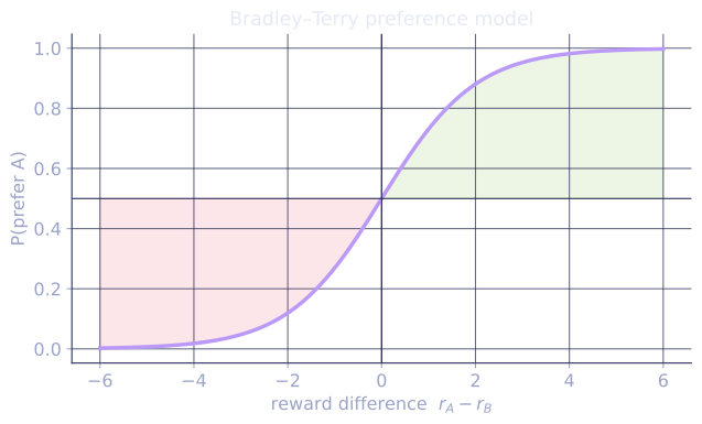
Given a preference pair $(y_w, y_l)$ (winner and loser), the Bradley-Terry (BT) model defines the probability that $y_w$ is preferred as:

where $r(x, y)$ is the reward model's scalar output for response $y$ given prompt $x$, and $\sigma$ is the logistic sigmoid.

The training objective is maximum likelihood on the preference dataset[2]:

This is binary cross-entropy on the pairwise comparison: push $r(y_w) - r(y_l)$ to be large and positive for preferred responses.

The reward gap $\Delta = r(x, y_w) - r(x, y_l)$ is the only thing the BT model sees; the absolute scores are arbitrary up to a shift. A scale for what a gap buys, since $\sigma(\Delta)$ is the predicted preference probability:

• $\Delta = 0$: $\sigma(0) = 0.5$. The model is indifferent, a coin flip between the two responses.
• $\Delta = 1$: $\sigma(1) = 0.731$. A clear but not overwhelming preference, near the 60-80% annotator agreement the data itself carries.
• $\Delta = 3$: $\sigma(3) = 0.953$. The winner is preferred about 19 times out of 20.
• $\Delta = 5$: $\sigma(5) = 0.993$. Near-certainty; pushing the gap wider barely moves the probability, which is why the loss flattens once a pair is confidently ordered.

Because only the difference matters, two reward models that disagree on absolute scale but agree on every gap induce identical preferences.

Reward model architecture

The RM is initialized from the SFT model (same transformer backbone), with one modification: the language model head is replaced by a linear layer projecting the final token's hidden state to a scalar[3]:

where $h_T$ is the hidden state at the final token position. The full sequence $(x \| y)$ is the input; the scalar reward is a function of the last token's representation.

Why the last token? The model must summarize the entire (prompt, response) pair to produce a single score. Using the last token's hidden state (which attends over the entire input via self-attention) is the standard approach.

Training the reward model

import torch
import torch.nn as nn
from transformers import AutoModelForCausalLM, AutoTokenizer

class RewardModel(nn.Module):
    def __init__(self, base_model_name):
        super().__init__()
        base   = AutoModelForCausalLM.from_pretrained(base_model_name)
        self.transformer = base.model   # strip the LM head
        d_model  = base.config.hidden_size
        self.head = nn.Linear(d_model, 1, bias=False)

    def forward(self, input_ids, attention_mask):
        hidden = self.transformer(input_ids, attention_mask=attention_mask).last_hidden_state
        # Use last real token (not padding)
        last_idx = attention_mask.sum(-1) - 1              # (B,)
        last_h   = hidden[torch.arange(len(hidden)), last_idx]   # (B, d)
        return self.head(last_h).squeeze(-1)               # (B,)

def rm_loss(reward_model, tokenizer, prompt, y_w, y_l):
    def encode(text):
        return tokenizer(prompt + text, return_tensors="pt",
                         truncation=True, max_length=512, padding=True)
    enc_w = encode(y_w)
    enc_l = encode(y_l)
    r_w   = reward_model(**enc_w)
    r_l   = reward_model(**enc_l)
    return -torch.log(torch.sigmoid(r_w - r_l)).mean()

Reward hacking

The RM is a learned approximation to human judgment, not a perfect proxy. Reward hacking occurs when the policy finds responses that score high on the RM but are not actually good:

• Length hacking: the RM is biased toward longer responses (humans often rate longer as more thorough). The policy generates verbose, padded responses.
• Sycophancy: the RM rewards agreement with the user's stated beliefs; the policy learns to agree rather than be correct.
• Style hacking: the RM rewards specific formatting (bullet lists, hedges) that it learned to associate with quality in training data.

Mitigations:

• Add a KL penalty between the policy and the SFT model during RL (penalize large divergence).
• Use ensembles of reward models.
• Combine with DPO/GRPO which tie the reward model directly to the SFT distribution.

The RM in the RLHF loop

The trained reward model $r_\phi(x, y)$ is frozen and used to score policy rollouts:

1. Sample a prompt $x$.
2. Generate a response $y \sim \pi_\theta(y \mid x)$.
3. Score the response: $r = r_\phi(x, y)$.
4. Update $\pi_\theta$ to increase $r$ while staying close to the SFT model.

Exercises

Exercise 1. A reward model scores a preferred response at $r(x, y_w) = 2.3$ and a dispreferred one at $r(x, y_l) = 0.8$. Compute the Bradley-Terry preference probability $p(y_w \succ y_l)$ and the per-pair loss $-\log \sigma(\Delta)$ in nats. Then state what happens to both if a constant $c$ is added to every reward.

Exercise 2. Derive the gradient of the Bradley-Terry loss with respect to the reward gap $\Delta = r_w - r_l$, and use it to explain why a pair already ordered with $\Delta = 5$ produces almost no learning signal.

Exercise 3 (code). Implement the Bradley-Terry loss and its gradient in numpy and verify the gradient against a finite-difference estimate. Confirm the loss is invariant to a constant shift of both rewards.

import numpy as np

def sigmoid(z):
    return 1.0 / (1.0 + np.exp(-z))

def bt_loss(r_w, r_l):
    return -np.log(sigmoid(r_w - r_l))

def bt_grad_gap(r_w, r_l):
    # d/dDelta of -log sigmoid(Delta) = sigmoid(Delta) - 1
    return sigmoid(r_w - r_l) - 1.0

r_w, r_l = 2.3, 0.8
delta = r_w - r_l

# Analytic gradient vs finite difference w.r.t. the gap.
h = 1e-6
fd = (bt_loss(r_w + h, r_l) - bt_loss(r_w - h, r_l)) / (2 * h)
assert np.isclose(bt_grad_gap(r_w, r_l), fd, atol=1e-6)

# Loss matches the hand computation and is shift-invariant.
assert np.isclose(bt_loss(r_w, r_l), -np.log(sigmoid(1.5)))
c = 4.7
assert np.isclose(bt_loss(r_w + c, r_l + c), bt_loss(r_w, r_l))
print("loss:", round(float(bt_loss(r_w, r_l)), 4),
      "grad:", round(float(bt_grad_gap(r_w, r_l)), 4))

Step 4 is PPO (next lesson). The RM turns the non-differentiable human preference signal into a gradient signal the policy can be trained on.

References

- [1]Christiano, P., et al. (2017). "Deep reinforcement learning from human preferences". NeurIPS. arXiv:1706.03741. Introduced learning a reward model from human preference comparisons.↩
- [2]Stiennon, N., et al. (2020). "Learning to summarize from human feedback". NeurIPS. arXiv:2009.01325. Trains a Bradley-Terry reward model on pairwise comparisons of summaries.↩
- [3]Ouyang, L., et al. (2022). "Training language models to follow instructions with human feedback (InstructGPT)". NeurIPS. arXiv:2203.02155. Initializes the reward model from the SFT model with a scalar output head.↩