Why ensembles work

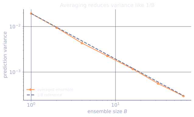
Bagging and boosting work for different reasons. Bagging lowers the variance of a high-variance learner by averaging across data perturbations. Boosting lowers the bias of a high-bias learner by sequentially fitting residuals. The common failure mode for both is correlated errors: if every base model makes the same mistake, no amount of averaging will correct it[1, 2].

The bias-variance reading

Recall the decomposition for squared loss at a test point: expected error = bias$^2$ + variance + noise.

Bagging. Averaging $B$ identically distributed predictors with pairwise correlation $\rho$ has variance[3]

As $B \to \infty$, the second term vanishes and only $\rho\sigma^2$ remains. Bagging works to the extent that:

1. Each base model has substantial variance to begin with (high-variance base learners like deep trees benefit most).
2. The base models are weakly correlated. Random forests reduce $\rho$ with random feature subsets; bagging on small datasets reduces it through bootstrap variation.

Bagging cannot reduce bias: an underfitting base model still underfits when averaged.

Boosting. Sequential boosting fits each new learner to the residuals (gradient) of the current ensemble. The training loss decreases at every step, driving down bias. Variance does not benefit (each round depends on the previous, so noise compounds rather than cancels). To prevent variance from growing, boosting uses weak learners (small bias contribution each) and a small learning rate (small step).

Correlated errors: the universal failure

Both methods fall apart when base models make the same mistakes:

• Bagging on deep trees with one dominant feature: every tree splits on it first, so they all agree on the dominant axis. The variance reduction on the dominant axis is small.
• Boosting on systematically mislabeled data: each round chases the same noise pattern.
• Stacking highly correlated base models: the meta-learner has no signal from any one model that the others lack.

The remedy is always diversity: different feature subsets (random forests), different model classes (stacking heterogeneous learners), different algorithms, different data subsets.

When ensembles do not help

Diminishing returns set in once:

• The base model is already low-variance (e.g. linear regression on a well-conditioned problem). Bagging adds noise without removing much.
• The base model is already low-bias (e.g. an unregularized deep network on a small problem). Boosting overfits without reducing bias.

A useful rule: ensembles improve a learner against its own failure mode. Use bagging on high-variance learners, boosting on high-bias ones, and stacking when you have multiple learners with complementary strengths.

Practical recipe

The standard tabular pipeline:

1. Random forest (bagged decorrelated trees) as a fast baseline. Good default; often surprisingly competitive.
2. Gradient boosting (XGBoost, LightGBM, CatBoost). Usually best single-model performance on tabular data.
3. Stacking (next lesson) when accuracy must be squeezed further by combining heterogeneous models.

Check it on arrays

import numpy as np

rng = np.random.default_rng(0)

# Toy regression: y = sin(x) + noise
def make_data(n=50, sigma=0.3, rng=rng):
    x = rng.uniform(0, 1, n)
    y = np.sin(2 * np.pi * x) + sigma * rng.normal(size=n)
    return x, y

# High-variance base learner: deep polynomial fit (overfit)
def fit_poly(x, y, degree):
    return np.polyfit(x, y, degree)

def predict_poly(coefs, x):
    return np.polyval(coefs, x)

x_test = np.linspace(0, 1, 100)
f_true = np.sin(2 * np.pi * x_test)

# Bias-variance of a single deep polynomial across many random datasets
single_preds = []
for t in range(200):
    x, y = make_data(rng=np.random.default_rng(1000 + t))
    coefs = fit_poly(x, y, degree=10)
    single_preds.append(predict_poly(coefs, x_test))
single_preds = np.array(single_preds)

bias_single = np.mean((single_preds.mean(axis=0) - f_true)**2)
var_single = np.mean(single_preds.var(axis=0))
print(f"single deep polynomial: bias^2 = {bias_single:.3f}, variance = {var_single:.3f}")

# Bagging: average over B bootstrap samples per dataset
B = 30
bagged_preds = []
for t in range(200):
    x, y = make_data(rng=np.random.default_rng(1000 + t))
    rng_in = np.random.default_rng(2000 + t)
    boot_preds = []
    for _ in range(B):
        idx = rng_in.integers(0, len(x), len(x))
        coefs = fit_poly(x[idx], y[idx], degree=10)
        boot_preds.append(predict_poly(coefs, x_test))
    bagged_preds.append(np.mean(boot_preds, axis=0))
bagged_preds = np.array(bagged_preds)

bias_bag = np.mean((bagged_preds.mean(axis=0) - f_true)**2)
var_bag = np.mean(bagged_preds.var(axis=0))
print(f"bagged deep polynomial: bias^2 = {bias_bag:.3f}, variance = {var_bag:.3f}  (variance ↓, bias same)")

# Boosting must use a weak learner whose model class genuinely expands when
# combined. Stumps (one-split piecewise constants) work; a sum of degree-1
# polynomials is still degree 1, so polynomial boosting cannot reduce bias.
def fit_stump(x, y):
    order = np.argsort(x); xs, ys = x[order], y[order]
    cum = np.cumsum(ys); n = len(ys); total = cum[-1]
    best = (None, None, None, np.inf)
    for k in range(1, n):
        thr = (xs[k - 1] + xs[k]) / 2
        sum_l, sum_r = cum[k - 1], total - cum[k - 1]
        mean_l, mean_r = sum_l / k, sum_r / (n - k)
        sse = np.sum((ys[:k] - mean_l)**2) + np.sum((ys[k:] - mean_r)**2)
        if sse < best[3]: best = (thr, mean_l, mean_r, sse)
    return best[:3]

def predict_stumps(stumps, x):
    F = np.zeros_like(x)
    for eta, (thr, ml, mr) in stumps:
        F = F + eta * np.where(x < thr, ml, mr)
    return F

def stagewise_fit_stumps(x, y, n_rounds=40, eta=0.3):
    F = np.zeros_like(y); stumps = []
    for _ in range(n_rounds):
        thr, ml, mr = fit_stump(x, y - F)
        stumps.append((eta, (thr, ml, mr)))
        F = F + eta * np.where(x < thr, ml, mr)
    return stumps

boost_preds = []
for t in range(200):
    x, y = make_data(rng=np.random.default_rng(1000 + t))
    stumps = stagewise_fit_stumps(x, y, n_rounds=40, eta=0.3)
    boost_preds.append(predict_stumps(stumps, x_test))
boost_preds = np.array(boost_preds)

bias_boost = np.mean((boost_preds.mean(axis=0) - f_true)**2)
var_boost = np.mean(boost_preds.var(axis=0))

# Bias of a single weak learner (one stump): much higher, so we can show the drop.
single_stump_preds = []
for t in range(200):
    x, y = make_data(rng=np.random.default_rng(1000 + t))
    thr, ml, mr = fit_stump(x, y)
    single_stump_preds.append(np.where(x_test < thr, ml, mr))
single_stump_preds = np.array(single_stump_preds)
bias_single_stump = np.mean((single_stump_preds.mean(axis=0) - f_true)**2)

print(f"single stump:    bias^2 = {bias_single_stump:.3f}")
print(f"boosted stumps:  bias^2 = {bias_boost:.3f}, variance = {var_boost:.3f}  (bias ↓ vs single stump)")

Bagging the deep polynomial cuts variance while leaving bias roughly unchanged; boosting stumps drops the bias far below a single stump because each round refits the residual with a fresh split.

Exercises

Exercise 1. Using the bagging variance formula $\rho\sigma^2 + \frac{1-\rho}{B}\sigma^2$, compute the variance of the averaged predictor for $\sigma^2 = 4$, $B = 25$, at $\rho = 0$ and at $\rho = 0.5$. What fraction of the original $\sigma^2$ remains in each case, and what does the comparison say about decorrelation?

Exercise 2. Derive the bagging variance formula. Let $\hat f_1, \dots, \hat f_B$ be identically distributed predictors, each with variance $\sigma^2$ and pairwise correlation $\rho$. Show that the average $\bar f = \frac{1}{B}\sum_b \hat f_b$ has variance $\rho\sigma^2 + \frac{1-\rho}{B}\sigma^2$.

Exercise 3 (code). Simulate $B$ identically distributed predictors with pairwise correlation $\rho$ (build them from a shared common factor) and verify empirically that the variance of their average matches the formula at several $(\rho, B)$ pairs, and that it approaches the $\rho\sigma^2$ floor as $B$ grows.

import numpy as np

rng = np.random.default_rng(0)

# X_b = sqrt(rho)*Z + sqrt(1-rho)*E_b, shared factor Z and private noise E_b,
# scaled by sigma. Then Var(X_b) = sigma^2 and Corr(X_i, X_j) = rho for i != j.
def correlated_predictors(B, rho, sigma, n_samples, rng):
    Z = rng.normal(size=(n_samples, 1))
    E = rng.normal(size=(n_samples, B))
    return (np.sqrt(rho) * Z + np.sqrt(1 - rho) * E) * sigma

sigma = 2.0
n_samples = 400_000
for rho, B in [(0.0, 10), (0.3, 10), (0.3, 50), (0.8, 50)]:
    X = correlated_predictors(B, rho, sigma, n_samples, rng)
    empirical = X.mean(axis=1).var()
    formula = rho * sigma**2 + (1 - rho) / B * sigma**2
    print(f"rho={rho}, B={B}: empirical={empirical:.4f}, formula={formula:.4f}")
    assert np.isclose(empirical, formula, rtol=0.03)

# As B grows with rho fixed, the average's variance approaches rho*sigma^2.
X_big = correlated_predictors(2000, 0.3, sigma, n_samples, rng)
floor = 0.3 * sigma**2
assert abs(X_big.mean(axis=1).var() - floor) < 0.05
print(f"large-B variance {X_big.mean(axis=1).var():.4f} -> floor {floor:.4f}")

The next lesson combines multiple learners explicitly via stacking.

References

- [1]Dietterich, T. G. (2000). "Ensemble methods in machine learning". Multiple Classifier Systems (MCS). Surveys why ensembles outperform single learners (doi:10.1007/3-540-45014-9_1).↩
- [2]Hansen, L. K., & Salamon, P. (1990). "Neural network ensembles". IEEE TPAMI, 12(10), 993-1001. Shows averaging independent classifiers reduces error when individual errors are uncorrelated (doi:10.1109/34.58871).↩
- [3]Breiman, L. (1996). "Bagging predictors". Machine Learning, 24(2), 123-140. Introduces bootstrap aggregation and the variance-reduction argument (doi:10.1007/BF00058655).↩