Train on TinyShakespeare

The block is the hard part. This lesson wraps a stack of blocks in the embedding and unembedding layers, defines the forward pass with its loss, adds autoregressive sampling, and runs the training loop from the setup lesson.

1. The full model

The model embeds token ids and positions, sums them into the residual stream, runs the blocks, applies a final LayerNorm, and projects to vocabulary logits. When targets are supplied it also returns the cross-entropy loss.

import torch
import torch.nn as nn
from torch.nn import functional as F

class GPTLanguageModel(nn.Module):
    def __init__(self, vocab_size, n_embd, n_head, n_layer, block_size, dropout=0.2):
        super().__init__()
        self.block_size = block_size
        self.token_embedding = nn.Embedding(vocab_size, n_embd)
        self.position_embedding = nn.Embedding(block_size, n_embd)
        self.blocks = nn.Sequential(
            *[Block(n_embd, n_head, block_size, dropout) for _ in range(n_layer)]
        )
        self.ln_f = nn.LayerNorm(n_embd)
        self.lm_head = nn.Linear(n_embd, vocab_size)

    def forward(self, idx, targets=None):
        B, T = idx.shape
        tok = self.token_embedding(idx)                          # (B,T,C)
        pos = self.position_embedding(torch.arange(T, device=idx.device))
        x = tok + pos                                            # (B,T,C)
        x = self.blocks(x)
        x = self.ln_f(x)
        logits = self.lm_head(x)                                 # (B,T,vocab)
        if targets is None:
            return logits, None
        B, T, V = logits.shape
        loss = F.cross_entropy(logits.view(B * T, V), targets.view(B * T))
        return logits, loss

The loss is cross-entropy over the flattened (B*T) predictions, which is the maximum likelihood objective for next-token prediction.

2. Autoregressive generation

Sampling feeds the model its own output one token at a time. Crop the context to the last block_size tokens, take the final-position logits, convert to probabilities, and sample.

@torch.no_grad()
def generate(model, idx, max_new_tokens):
    for _ in range(max_new_tokens):
        idx_cond = idx[:, -model.block_size :]
        logits, _ = model(idx_cond)
        logits = logits[:, -1, :]                 # last position only
        probs = F.softmax(logits, dim=-1)
        next_id = torch.multinomial(probs, num_samples=1)
        idx = torch.cat((idx, next_id), dim=1)
    return idx

3. Run it

A small configuration trains in minutes on a GPU and still learns clear word shapes, punctuation, and speaker labels[1], the same character-level setup GPT-2 scaled to web text[2].

model = GPTLanguageModel(
    vocab_size=vocab_size, n_embd=384, n_head=6, n_layer=6,
    block_size=block_size, dropout=0.2,
).to(device)

train(model, max_iters=5000, eval_interval=500, lr=3e-4)   # from the setup lesson

start = torch.zeros((1, 1), dtype=torch.long, device=device)
print(decode(generate(model, start, max_new_tokens=500)[0].tolist()))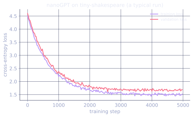

4. Reading the curves

Two things to watch. Train and validation loss both fall well below the uniform baseline of $\ln(\text{vocab\_size}) \approx 4.17$, confirming the model uses context. As training continues, validation loss flattens and then drifts up while train loss keeps falling: that gap is overfitting, the bias-variance tradeoff showing up in a transformer, and it is what dropout and weight decay hold back.

Exercises

Exercise 1. §4 reads the cross-entropy loss directly. A more interpretable companion is perplexity, $\text{ppl} = e^{\mathcal{L}}$ (with natural-log loss). Compute the perplexity of the uniform baseline $\mathcal{L} = \ln(65) \approx 4.17$, and interpret what perplexity means operationally for a character-level model.

Exercise 2 (code). Verify the loss-to-perplexity correspondence and the uniform baseline in numpy. Confirm that the perplexity of the uniform model over $65$ characters is exactly $65$, and that a sharper predicted distribution gives a lower perplexity.

import numpy as np

V = 65

# Uniform model: cross-entropy is ln(V), perplexity is V.
uniform_loss = np.log(V)
uniform_ppl = np.exp(uniform_loss)
assert np.isclose(uniform_ppl, V)

# A confident, mostly-correct model: put most mass on the true class.
true = 7
probs = np.full(V, 0.001)
probs[true] = 1.0 - 0.001 * (V - 1)
confident_loss = -np.log(probs[true])
confident_ppl = np.exp(confident_loss)

assert confident_ppl < uniform_ppl
print("uniform perplexity:  ", round(float(uniform_ppl), 4))
print("confident perplexity:", round(float(confident_ppl), 4))

Exercise 3 (code). The generate function samples the next token from the softmax of the final-position logits. Reproduce that sampling step in numpy: softmax a logit vector, draw many samples, and verify the empirical frequencies converge to the softmax probabilities, confirming torch.multinomial samples from the predicted distribution.

import numpy as np

rng = np.random.default_rng(0)

def softmax(z):
    z = z - z.max()
    e = np.exp(z)
    return e / e.sum()

V = 6
logits = rng.standard_normal(V)
probs = softmax(logits)

# Sample many next-token draws from the categorical distribution.
draws = rng.choice(V, size=200_000, p=probs)
freqs = np.bincount(draws, minlength=V) / len(draws)

# Empirical frequencies match the softmax probabilities to sampling tolerance.
assert np.allclose(freqs, probs, atol=0.01)
print("softmax probs:", np.round(probs, 4))
print("empirical:    ", np.round(freqs, 4))

The output at this point is recognizably Shakespeare-shaped but the architecture is the 2017 design. The next lesson modernizes it with RoPE and RMSNorm.

References

- [1]Karpathy, A. (2022). nanoGPT. GitHub repository, github.com/karpathy/nanoGPT. The TinyShakespeare training configuration followed here.↩
- [2]Radford, A., Wu, J., Child, R., Luan, D., Amodei, D., & Sutskever, I. (2019). "Language models are unsupervised multitask learners (GPT-2)". OpenAI. The same autoregressive objective at scale.↩