Smoothing and back-off

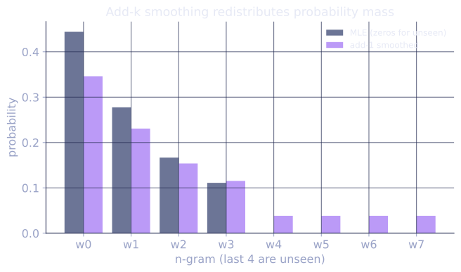
The MLE bigram assigns probability zero to any pair never seen in training. One unseen bigram in a test sentence collapses the entire sentence probability to zero and the perplexity to $+\infty$. Smoothing redistributes a portion of the probability mass from seen n-grams to unseen ones, so that every grammatical sentence receives a positive score[2, 3].

Laplace add-one smoothing

The simplest fix: pretend each n-gram was seen one extra time.

where $V$ is the vocabulary size (the $+V$ in the denominator ensures each row still sums to 1).

Every unseen bigram now gets probability $1 / (c(a) + V)$. The cost is heavy over-assignment: for a rare context $a$ with $c(a) = 2$ and $V = 50{,}000$, the pseudocount of 1 inflates the mass on unseen events to $50{,}000 / 50{,}002 \approx 99.9\%$ of the row's probability.

Add-one is useful as a pedagogical baseline but too aggressive for any practical use.

Discounting and redistribution

A better approach: reduce the counts of seen events by a small amount $d$, and pool the recovered mass into a "leftover" budget distributed to unseen events. This is the principle behind all practical smoothing methods.

Define the discounted count $c^*(a, b) = c(a, b) - d$ for some $0 < d < 1$. The discounted probability is:

The total mass removed from row $a$ is:

where $N_1(a)$ is the number of distinct words $b$ with $c(a,b) \ge 1$. This leftover mass $\lambda(a)$ is redistributed to unseen bigrams by a back-off distribution.

Kneser-Ney smoothing

Kneser-Ney (KN) is the best-performing classical smoother; it was the standard for over a decade[1]. The key innovation is the back-off distribution $p_{\text{KN}}(b)$: instead of using the unigram frequency of $b$, use the continuation probability, the number of distinct contexts in which $b$ appears.

Words like "York" have high unigram frequency but only appear after "New", so their continuation count is low. Words like "the" appear in many different contexts, so their continuation count is high. The continuation probability is a much better estimate of "how useful is $b$ as a completion when we have never seen the context."

The full interpolated KN bigram:

For higher-order n-grams, the interpolation recurses: the trigram backs off to the KN bigram, which backs off to the KN unigram.

Back-off vs interpolation

Two redistribution strategies:

Back-off (Katz 1987): use the discounted n-gram probability when the count is nonzero; fall back to the $(n-1)$-gram otherwise, weighted by a normalizing factor.

Interpolation: always take a weighted sum of all orders $1, \dots, n$, regardless of whether the n-gram was seen. Interpolation consistently outperforms pure back-off; KN uses interpolation.

Implementing Laplace and measuring perplexity

import numpy as np
from collections import Counter, defaultdict

corpus = [
    ["<bos>", "I", "am", "Sam", "<eos>"],
    ["<bos>", "Sam", "I", "am", "<eos>"],
    ["<bos>", "I", "do", "not", "like", "green", "eggs", "<eos>"],
]
unigrams = Counter(w for sent in corpus for w in sent)
bigrams  = Counter((a, b) for sent in corpus for a, b in zip(sent, sent[1:]))
V = len(unigrams)

def p_mle(a, b):
    return bigrams[(a, b)] / unigrams[a] if unigrams[a] else 0.0

def p_add1(a, b):
    return (bigrams[(a, b)] + 1) / (unigrams[a] + V)

def perplexity(model_p, test_sentences):
    log_prob, n = 0.0, 0
    for sent in test_sentences:
        for a, b in zip(sent, sent[1:]):
            log_prob += np.log(model_p(a, b) + 1e-300)
            n += 1
    return np.exp(-log_prob / n)

test = [
    ["<bos>", "I", "like", "ham", "<eos>"],   # contains unseen "I like"
    ["<bos>", "Sam", "I", "am", "<eos>"],
]

print(f"MLE perplexity:   {perplexity(p_mle,  test):.1f}")   # inf due to "I like"
print(f"Add-1 perplexity: {perplexity(p_add1, test):.1f}")   # finite

The MLE model returns $+\infty$ because "I like" was unseen. Add-one fixes this at the cost of significant probability distortion: each seen bigram has its probability shrunk to allocate mass to the vast space of unseen events.

What smoothing cannot fix

No smoothing method overcomes the fixed-range structural limit. Redistributing mass among unseen bigrams says nothing about which unseen bigrams are more likely; that requires generalizing through the geometry of word representations, which is exactly what embedding-based neural models provide.

Exercises

Exercise 1. A context $a$ has $c(a) = 4$ and a vocabulary of $V = 6$. The only bigram seen with this context is $(a, b)$ with $c(a, b) = 4$. Compute $\hat{p}_{\text{add-1}}(b \mid a)$ and $\hat{p}_{\text{add-1}}(b' \mid a)$ for any unseen $b'$, and check that the row sums to 1.

Exercise 2. Kneser-Ney replaces the unigram back-off with the continuation probability $p_{\text{KN}}(b) \propto |\{a : c(a, b) > 0\}|$. Take a corpus where "York" appears 100 times but always after "New", and "city" appears 40 times after 12 distinct words. Which word has the larger continuation probability, and why is that the behavior KN wants?

Exercise 3 (code). On the toy corpus, build add-one and MLE bigram models. Verify that the MLE assigns probability 0 to the unseen bigram ("I", "like") while add-one assigns it a positive probability, and that the add-one row for context "I" still sums to 1.

import numpy as np
from collections import Counter

corpus = [
    ["<bos>", "I", "am", "Sam", "<eos>"],
    ["<bos>", "Sam", "I", "am", "<eos>"],
    ["<bos>", "I", "do", "not", "like", "green", "eggs", "<eos>"],
]
unigrams = Counter(w for sent in corpus for w in sent)
bigrams = Counter((a, b) for sent in corpus for a, b in zip(sent, sent[1:]))
V = len(unigrams)
vocab = list(unigrams)

def p_mle(a, b):
    return bigrams[(a, b)] / unigrams[a] if unigrams[a] else 0.0

def p_add1(a, b):
    return (bigrams[(a, b)] + 1) / (unigrams[a] + V)

# "I like" never occurs in training
assert p_mle("I", "like") == 0.0
assert p_add1("I", "like") > 0.0

# Add-one row for context "I" sums to 1 over the full vocabulary
row_sum = sum(p_add1("I", w) for w in vocab)
assert np.isclose(row_sum, 1.0)
print("p_mle(I->like) =", p_mle("I", "like"),
      " p_add1(I->like) =", round(p_add1("I", "like"), 4),
      " row sum =", round(row_sum, 4))

The next lesson introduces BPE subword tokenization, which is a prerequisite for any neural LM.

References

- [1]Chen, S. F., & Goodman, J. (1999). "An empirical study of smoothing techniques for language modeling". Computer Speech & Language, 13(4), 359-394. The definitive comparison; establishes interpolated Kneser-Ney as the strongest classical method. doi:10.1006/csla.1999.0128↩
- [2]Manning, C. D., & Schütze, H. (1999). Foundations of Statistical Natural Language Processing. MIT Press. Discounting, back-off, and interpolation.↩
- [3]Jurafsky, D., & Martin, J. H. (2024). Speech and Language Processing (3rd ed. draft). Smoothing of n-gram models.↩