Information retrieval: TF-IDF and BM25

Information retrieval (IR) is the problem of ranking documents by relevance to a query. Before dense neural retrieval (E6), sparse lexical methods dominated: rank documents by how well their term frequencies match the query, with rarer terms weighted more heavily[1].

Term frequency

The simplest relevance signal: how often does a query term appear in a document?

Problem: a document that mentions "neural" 100 times is probably not 100x more relevant than one that mentions it once. Raw frequency overweights long documents and saturates quickly.

Inverse document frequency

Rare terms are more informative than common ones. "The" appears in every document and carries no discriminative signal. The inverse document frequency downweights terms proportional to their corpus-wide frequency:

where $N$ is the number of documents and $\text{df}(t)$ is the number of documents containing $t$. The $+1$ avoids division by zero for unseen terms.

Derivation from information theory. A term that appears in fraction $p = \text{df}(t)/N$ of documents has self-information $\log(1/p) = \log(N/\text{df}(t))$: rare terms carry more information per occurrence. IDF is this self-information.

A magnitude scale on a million-document corpus ($N = 10^6$) shows the weighting at work, using $\log(N/(1+\text{df}))$:

• A term in every document ("the", $\text{df} = N$): $\log(N/N) \approx 0$. No discriminative signal, so IDF zeroes it out.
• A term in half the corpus ($\text{df} = 5 \times 10^5$): $\log 2 \approx 0.69$.
• A term in 1% ($\text{df} = 10^4$): $\log 100 \approx 4.6$.
• A near-unique term ($\text{df} = 100$): $\log(10^4) \approx 9.2$.

So the gap between a stopword and a rare technical term is a factor of roughly $9.2 / 0.69 \approx 13$ in IDF weight, before TF even enters. The IDF spread is what makes a query's rare terms dominate its score.

TF-IDF

The TF-IDF weight of a term $t$ in document $d$ is:

Document relevance for query $q$: $\text{score}(q, d) = \sum_{t \in q} \text{TF-IDF}(t, d)$.

BM25

TF-IDF has two known failure modes:

1. No TF saturation. A document with 1000 occurrences of a term scores 1000x higher than one with 1 occurrence, even though relevance barely increases beyond a few repetitions.
2. No length normalization. Longer documents accumulate higher raw TF for every term.

BM25 fixes both[2]:

where:

• $\text{tf}(t, d)$ is the raw term frequency (count) in document $d$.
• $|d|$ is the document length in tokens; $\text{avgdl}$ is the average document length.
• $k_1 \in [1.2, 2.0]$ controls TF saturation: as $\text{tf} \to \infty$, the score approaches $\text{IDF}(t) \cdot (k_1 + 1)$, a finite ceiling.
• $b \in [0, 1]$ controls length normalization: $b=0$ disables it, $b=1$ fully normalizes.

Typical defaults: $k_1 = 1.5$, $b = 0.75$.

TF saturation. The term $\frac{\text{tf} \cdot (k_1+1)}{\text{tf} + k_1(\dots)}$ is a concave, saturating function of tf. At tf=0 it equals 0; as tf $\to \infty$ it approaches $k_1 + 1$. With $k_1 = 1.5$, the ceiling is 2.5 regardless of how many times the term appears.

Inverted index

Efficient retrieval precomputes an inverted index: for each term $t$, store a postings list of $(d, \text{tf})$ pairs for all documents containing $t$.

At query time:

1. Tokenize and normalize the query.
2. Look up each query term in the index to retrieve its postings list.
3. Merge the lists (union for OR, intersection for AND) and score each document.

import numpy as np
from collections import defaultdict, Counter
import math

docs = {
    "d1": "the quick brown fox jumps over the lazy dog",
    "d2": "the fox is quick and agile",
    "d3": "lazy animals sleep all day and night",
    "d4": "the dog chased the quick brown fox",
}

# Build inverted index
def tokenize(text):
    return text.lower().split()

index = defaultdict(list)   # term -> [(doc_id, tf)]
doc_lengths = {}
for doc_id, text in docs.items():
    tokens = tokenize(text)
    doc_lengths[doc_id] = len(tokens)
    tf = Counter(tokens)
    for term, count in tf.items():
        index[term].append((doc_id, count))

N = len(docs)
avgdl = np.mean(list(doc_lengths.values()))
k1, b = 1.5, 0.75

def idf(term):
    df = len(index.get(term, []))
    return math.log((N - df + 0.5) / (df + 0.5) + 1)

def bm25_score(query, doc_id, doc_length, index):
    score = 0.0
    for term in tokenize(query):
        postings = {d: tf for d, tf in index.get(term, [])}
        tf = postings.get(doc_id, 0)
        score += idf(term) * (tf * (k1 + 1)) / (tf + k1 * (1 - b + b * doc_length / avgdl))
    return score

query = "quick fox"
scores = {doc_id: bm25_score(query, doc_id, doc_lengths[doc_id], index)
          for doc_id in docs}
ranked = sorted(scores.items(), key=lambda x: -x[1])
for doc_id, score in ranked:
    print(f"  {doc_id} ({score:.3f}): {docs[doc_id]}")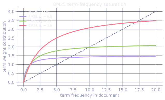

Exercises

Exercise 1. A corpus has $N = 1000$ documents. Term "neural" appears in $\text{df} = 10$ of them; term "the" appears in all $1000$. Using the lesson's IDF definition $\text{IDF}(t) = \log\frac{N}{1 + \text{df}(t)}$ (natural log), compute both IDF weights and the ratio between them.

Exercise 2. BM25's TF factor is $\frac{\text{tf}(k_1 + 1)}{\text{tf} + k_1(1 - b + b \cdot |d|/\text{avgdl})}$. For a document of average length ($|d| = \text{avgdl}$) with $k_1 = 1.5$, $b = 0.75$, compute the TF factor at $\text{tf} = 1$ and at $\text{tf} = 10$, and the saturation ceiling as $\text{tf} \to \infty$.

Exercise 3 (code). Build a small inverted index over four documents and rank them for the query "quick fox" with BM25. Confirm that the documents containing both query terms outrank those containing only one, and that any document containing neither term scores exactly 0.

import numpy as np
from collections import defaultdict, Counter
import math

docs = {
    "d1": "the quick brown fox jumps over the lazy dog",
    "d2": "the fox is quick and agile",
    "d3": "lazy animals sleep all day and night",   # neither query term
    "d4": "the dog chased the quick brown fox",
}

def tokenize(text):
    return text.lower().split()

index = defaultdict(list)
doc_lengths = {}
for doc_id, text in docs.items():
    tokens = tokenize(text)
    doc_lengths[doc_id] = len(tokens)
    for term, count in Counter(tokens).items():
        index[term].append((doc_id, count))

N = len(docs)
avgdl = np.mean(list(doc_lengths.values()))
k1, b = 1.5, 0.75

def idf(term):
    df = len(index.get(term, []))
    return math.log((N - df + 0.5) / (df + 0.5) + 1)

def bm25_score(query, doc_id):
    score = 0.0
    for term in tokenize(query):
        postings = {d: tf for d, tf in index.get(term, [])}
        tf = postings.get(doc_id, 0)
        L = doc_lengths[doc_id]
        score += idf(term) * (tf * (k1 + 1)) / (tf + k1 * (1 - b + b * L / avgdl))
    return score

scores = {d: bm25_score("quick fox", d) for d in docs}

# d3 has neither "quick" nor "fox": exact zero
assert scores["d3"] == 0.0
# d1, d2, d4 all contain both terms; each beats d3
for d in ["d1", "d2", "d4"]:
    assert scores[d] > scores["d3"]
print({d: round(s, 3) for d, s in sorted(scores.items(), key=lambda x: -x[1])})

Sparse retrieval in the LLM era

BM25 remains the backbone of production search engines (Elasticsearch, OpenSearch). Modern retrieval-augmented generation (RAG) pipelines often combine BM25 (lexical, exact-match) with dense neural retrieval (semantic, embedding-based) using reciprocal rank fusion to blend their ranked lists. BM25 handles precise keyword matches (product SKUs, proper nouns) better than dense retrievers, making hybrid retrieval a practical default.

References

- [1]Manning, C. D., Raghavan, P., & Schütze, H. (2008). Introduction to Information Retrieval. Cambridge University Press. TF-IDF weighting, the vector space model, and inverted indexes.↩
- [2]Robertson, S., & Zaragoza, H. (2009). "The probabilistic relevance framework: BM25 and beyond". Foundations and Trends in Information Retrieval, 3(4), 333-389. The derivation and tuning of the BM25 saturation and length-normalization terms. doi:10.1561/1500000019↩