Convolution and pooling

Images have local structure and translation invariance: a cat edge looks the same wherever it appears in the image, and pixels matter relative to their neighbors. A fully connected MLP throws this away by mixing every input with every output. Convolution exploits both: the same small filter is applied at every location, drastically cutting parameters and bringing the inductive bias of "local + translation- equivariant" into the network[1, 2].

The 2D convolution

Given an input feature map $X \in \mathbb{R}^{H \times W \times C_{\text{in}}}$ and a filter $K \in \mathbb{R}^{k_h \times k_w \times C_{\text{in}} \times C_{\text{out}}}$, the output at position $(i, j, c)$ is

Three pieces: a spatial window of size $k_h \times k_w$ at each output location, a per-channel inner product with the filter, and a bias per output channel.

The filter $K$ has $k_h k_w C_{\text{in}} C_{\text{out}}$ weights, shared across every spatial location. For a $256 \times 256$ image with 64 output channels and $3 \times 3$ filters, the layer has $3 \cdot 3 \cdot C_{\text{in}} \cdot 64$ weights regardless of image size, where a fully connected equivalent would have $256 \cdot 256 \cdot C_{\text{in}} \cdot 64$.

Stride and padding

Stride $s$ moves the window by $s$ positions instead of 1, downsampling the output. Output spatial size becomes $\lfloor (H - k_h)/s \rfloor + 1$.

Padding adds zeros around the input border. "Same" padding chooses padding so the output has the same spatial size as the input (for stride 1); "valid" padding uses none.

These two knobs control the receptive field and the spatial dimensions through the network.

Receptive field

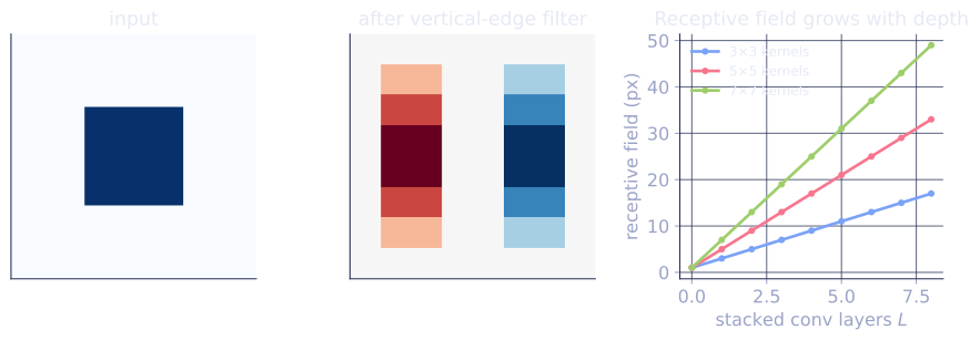
Each output unit depends on a small patch of the input through one convolution. Stacking $L$ convolutions of size $k$ each gives a receptive field of size $1 + L(k - 1)$ on the input. Strided convolutions and pooling expand the receptive field much faster (multiplicatively).

By design, deep CNNs grow their receptive field from local edges to whole-image features as you go up the layer stack: early layers see 3-pixel patches, deep layers see hundreds of pixels.

Why convolution and not full mixing

Three inductive biases for free:

• Locality: the output at position $(i, j)$ depends only on a small patch around $(i, j)$.
• Translation equivariance: shifting the input shifts the output by the same amount. A cat is a cat wherever it appears.
• Parameter sharing: the same filter is used at every location, cutting parameters by orders of magnitude.

For natural images these biases are correct, and a CNN with one tenth of an MLP's parameters typically far outperforms it. For other domains (tabular data), the locality assumption is wrong and convolutions are inappropriate.

Pooling

After convolution, pooling downsamples the spatial dimensions while keeping the channel dimension:

• Max pooling: take the max within each window. Preserves the strongest activation, robust to small shifts.
• Average pooling: take the mean within each window. Smoother.
• Global average pooling: average over the entire spatial extent, collapsing $H \times W \times C$ to $C$. Used at the end of a CNN before the classifier head.

Modern architectures sometimes drop pooling in favor of strided convolutions (the convolution itself does the downsampling). They are nearly equivalent.

Padding details

• Causal padding (1D): pad only on the past side. Used in WaveNet and time-series CNNs.
• Reflection / replication padding: instead of zero. Reduces edge artifacts in image generation networks.
• Symmetric vs asymmetric: filter sizes are typically odd ($3, 5, 7$) so the same padding on each side works cleanly.

Channels

The channel axis is the truly important one: it carries the learned features. A $3 \times 3 \times 64 \to 3 \times 3 \times 128$ layer mixes 128 output features from 64 input features at every location.

CNNs commonly:

• Start with few channels (e.g. 64) matching the image's 3 RGB inputs.
• Double channels every time spatial dimensions halve, keeping the feature volume roughly constant.
• End with many channels (256-2048) feeding into a small spatial extent that gets globally pooled into a vector for the classifier.

Check it on arrays

import numpy as np

rng = np.random.default_rng(0)

def conv2d(X, K, stride=1, pad=0):
    """Naive 2D convolution. X: (H, W, Cin). K: (kh, kw, Cin, Cout)."""
    if pad > 0:
        X = np.pad(X, ((pad, pad), (pad, pad), (0, 0)))
    H, W, Cin = X.shape
    kh, kw, _, Cout = K.shape
    out_h = (H - kh) // stride + 1
    out_w = (W - kw) // stride + 1
    Y = np.zeros((out_h, out_w, Cout))
    for i in range(out_h):
        for j in range(out_w):
            patch = X[i*stride:i*stride+kh, j*stride:j*stride+kw, :]   # (kh, kw, Cin)
            Y[i, j, :] = np.tensordot(patch, K, axes=([0, 1, 2], [0, 1, 2]))
    return Y

# Single-channel input, edge-detection filter
X = np.zeros((10, 10, 1))
X[3:7, 3:7, 0] = 1.0                                # white square on black

# Vertical-edge filter
K_vert = np.array([[-1, 0, 1], [-1, 0, 1], [-1, 0, 1]]).reshape(3, 3, 1, 1).astype(float)
Y = conv2d(X, K_vert)
print(f"input shape  {X.shape},  output shape {Y.shape}")
print("vertical-edge response (rounded):")
print(Y[:, :, 0].astype(int))

# Stride and padding effects on output spatial size
for stride in [1, 2]:
    for pad in [0, 1]:
        out = conv2d(X, K_vert, stride=stride, pad=pad)
        print(f"stride={stride}, pad={pad}: output {out.shape[:2]}")

# Max pooling
def max_pool2d(X, k=2, stride=2):
    H, W, C = X.shape
    out_h = (H - k) // stride + 1
    out_w = (W - k) // stride + 1
    Y = np.zeros((out_h, out_w, C))
    for i in range(out_h):
        for j in range(out_w):
            patch = X[i*stride:i*stride+k, j*stride:j*stride+k, :]
            Y[i, j, :] = patch.max(axis=(0, 1))
    return Y

pooled = max_pool2d(X)
print(f"\nmax pool 2x2 stride 2: {X.shape} -> {pooled.shape}")

The vertical-edge filter lights up at the left and right sides of the white square (positive and negative responses respectively); pooling halves the spatial dimensions.

Exercises

Exercise 1. An input feature map is $32 \times 32$. A convolution uses a $5 \times 5$ filter with stride $2$ and padding $1$. Compute the output spatial size by hand.

Exercise 2. A network stacks $L$ convolutions, each $k \times k$ with stride $1$ and no pooling. Derive the receptive field size $1 + L(k - 1)$, then find how many $3 \times 3$ layers are needed for one output unit to see a $15 \times 15$ region of the input.

Exercise 3 (code). Implement the output-size formula and verify it against the conv2d from the lesson: for a $7 \times 7$ single-channel input with a $3 \times 3$ filter at stride $2$, padding $1$, the formula and the actual output shape must agree.

import numpy as np

def conv2d(X, K, stride=1, pad=0):
    if pad > 0:
        X = np.pad(X, ((pad, pad), (pad, pad), (0, 0)))
    H, W, Cin = X.shape
    kh, kw, _, Cout = K.shape
    out_h = (H - kh) // stride + 1
    out_w = (W - kw) // stride + 1
    Y = np.zeros((out_h, out_w, Cout))
    for i in range(out_h):
        for j in range(out_w):
            patch = X[i*stride:i*stride+kh, j*stride:j*stride+kw, :]
            Y[i, j, :] = np.tensordot(patch, K, axes=([0, 1, 2], [0, 1, 2]))
    return Y

def out_size(H, k, stride, pad):
    return (H + 2 * pad - k) // stride + 1

rng = np.random.default_rng(0)
X = rng.normal(size=(7, 7, 1))
K = rng.normal(size=(3, 3, 1, 1))

predicted = out_size(7, 3, stride=2, pad=1)          # (7 + 2 - 3)//2 + 1 = 4
actual = conv2d(X, K, stride=2, pad=1).shape[0]
assert predicted == actual == 4
print("predicted:", predicted, " actual:", actual)

The next lesson stacks these primitives into the classic CNN architectures.

References

- [1]LeCun, Y., Bottou, L., Bengio, Y., & Haffner, P. (1998). "Gradient-based learning applied to document recognition". Proceedings of the IEEE, 86(11), 2278-2324. doi:10.1109/5.726791. Introduces the convolution-pooling stack with shared filters.↩
- [2]Goodfellow, I., Bengio, Y., & Courville, A. (2016). Deep Learning, §9 (Convolutional Networks). MIT Press. Locality, parameter sharing, and equivariance as the convolutional inductive biases.↩