 AI Knowledge Tree
Classic CNN architectures
Trace LeNet, AlexNet, VGG, and ResNet's skip connections, and see why depth without residuals collapses gradient flow.
Image classification went from "hard problem" to "approximately solved" in less than a decade because of four architectures: LeNet (1998) established the convolution-pooling stack; AlexNet (2012) scaled it with ReLUs and GPUs; VGG (2014) showed depth alone helped; ResNet (2015) unlocked truly deep networks with skip connections. Every modern CNN is a refinement of the ResNet pattern.
LeNet (1998)
LeCun's original convolutional network for digit recognition[1]:
input (32x32x1)
  -> conv 5x5, 6 filters    -> relu -> avg pool 2x2
  -> conv 5x5, 16 filters   -> relu -> avg pool 2x2
  -> fc 120 -> relu
  -> fc 84  -> relu
  -> fc 10  -> softmax
Two convolutional blocks, three fully connected layers. About 60K parameters. Trained on MNIST to 99% accuracy. The blueprint for every CNN that followed: stack convolutions, downsample with pooling, flatten, classify.
AlexNet (2012)
Krizhevsky et al.'s ImageNet winner[2]. The "ResNet moment" for the field.
Key changes from LeNet:
- 5 conv layers + 3 fc layers, ~60M parameters.
- ReLU instead of sigmoid/tanh (the dead-ReLU lesson).
- GPU training: two GPUs, splitting the model across them.
- Dropout in the fc layers.
- Data augmentation: random crops and horizontal flips.
- Local response normalization (a precursor to batch norm).
Trained on 1.2M ImageNet images to a top-5 error of 15.3%, halving the previous state of the art. The result triggered the deep-learning boom.
VGG (2014)
Simonyan and Zisserman replaced AlexNet's mix of filter sizes with a uniform stack of convolutions[3]:
[conv 3x3 x 2] -> pool
[conv 3x3 x 2] -> pool
[conv 3x3 x 3] -> pool
[conv 3x3 x 3] -> pool
[conv 3x3 x 3] -> pool
fc 4096 -> fc 4096 -> fc 1000
Two design choices proved durable:
- Small filters stacked: two convolutions have the same receptive field as one , but with fewer parameters and an extra nonlinearity. Three s match a .
- Channel doubling at each spatial downsample: feature volume stays roughly constant.
VGG-16 and VGG-19 are deeper variants. Reached 7.3% top-5 error on ImageNet. The architecture is heavyweight (138M parameters) but conceptually clean and still used as a feature extractor in many vision papers.
The depth-collapse problem
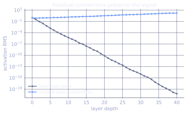
Going from VGG-19 to "plain VGG-30 or 50" should help: more depth, more capacity, lower training error. Instead, training error increases as plain networks get deeper past ~20 layers.
The diagnosis is not overfitting (training error is the wrong thing for that). It is an optimization problem: gradients propagate poorly through very deep stacks of compositions, and the network gets stuck in a region where it cannot even learn the identity function on each sublayer.
ResNet's contribution was to fix this directly.
ResNet (2015)
He et al.'s residual block[4]:
The output is the sum of a learned (typically a stack of 2 or 3 convolutions with BatchNorm and ReLU) and a shortcut connection that bypasses entirely.
The crucial property: now has to learn the difference between the input and the desired output, not the full mapping. If the right answer is the identity (do nothing), can be the zero function and the block degenerates to the identity. Training error stops increasing with depth.
A ResNet-50 has 50 layers; ResNet-152 has 152. Both train without collapse and beat VGG-19 substantially on ImageNet.
Why residual works (briefly)
Several explanations, all partially right:
- Gradient flow: the shortcut connection provides a path that preserves the gradient regardless of how badly behaves. Backpropagation through gives ; the term passes through unscaled.
- Loss landscape smoothing: empirical work shows residual nets have much smoother loss landscapes than plain ones.
- Ensembling: a -layer ResNet behaves like an ensemble of paths of varying depths (any subset of residual blocks can be active).
Whichever explanation, the empirical fact is overwhelming: residual connections are the single architectural change that made very deep networks trainable, and they appear in every architecture since (Transformers, U-Nets, diffusion backbones, you name it).
The classic recipe at a glance
| Year | Network | Layers | Params | Top-5 ImageNet error |
|---|---|---|---|---|
| 1998 | LeNet-5 | 7 | 60K | (MNIST, ~1% err) |
| 2012 | AlexNet | 8 | 60M | 15.3% |
| 2014 | VGG-19 | 19 | 144M | 7.3% |
| 2015 | ResNet-152 | 152 | 60M | 3.6% |
| 2017 | DenseNet-201 | 201 | 20M | 4.7% |
| 2019 | EfficientNet-B7 | ~50 | 66M | 3.5% |
ResNet-152 simultaneously went deeper, smaller, and more accurate than VGG-19. The next lesson surveys what came after: DenseNet, EfficientNet, ConvNeXt.
Check it on arrays
import numpy as np

rng = np.random.default_rng(0)

def conv2d(X, K, stride=1, pad=0):
    if pad: X = np.pad(X, ((pad,pad),(pad,pad),(0,0)))
    H, W, _ = X.shape
    kh, kw, _, Co = K.shape
    out_h = (H - kh) // stride + 1; out_w = (W - kw) // stride + 1
    Y = np.zeros((out_h, out_w, Co))
    for i in range(out_h):
        for j in range(out_w):
            Y[i, j] = np.tensordot(X[i*stride:i*stride+kh, j*stride:j*stride+kw], K, axes=([0,1,2],[0,1,2]))
    return Y

def relu(x): return np.maximum(0, x)

# A residual block: y = relu(conv2(relu(conv1(x))) + x)
def residual_block(X, W1, W2, b1, b2):
    h = relu(conv2d(X, W1, pad=1) + b1)
    h = conv2d(h, W2, pad=1) + b2
    return relu(h + X)                           # shortcut

# Compare gradient norm through depth: plain vs residual
def plain_block(X, W1, W2, b1, b2):
    h = relu(conv2d(X, W1, pad=1) + b1)
    h = relu(conv2d(h, W2, pad=1) + b2)
    return h

C = 8
X = rng.normal(size=(16, 16, C))
def make_W(out_C=C): return rng.normal(scale=0.1, size=(3, 3, C, out_C))

for D in [1, 5, 10, 20]:
    h_plain = X.copy(); h_res = X.copy()
    Ws = [(make_W(), make_W(), np.zeros(C), np.zeros(C)) for _ in range(D)]
    for W1, W2, b1, b2 in Ws:
        h_plain = plain_block(h_plain, W1, W2, b1, b2)
        h_res   = residual_block(h_res, W1, W2, b1, b2)
    print(f"depth {D:>2}: plain output norm = {np.linalg.norm(h_plain):.3e}, "
          f"residual = {np.linalg.norm(h_res):.3e}")
Plain networks collapse their activation norm to near zero as depth grows because the small initialization compounds; residual networks preserve the norm via the shortcut.
Exercises
Exercise 1. VGG's design replaces one convolution with two stacked convolutions of the same receptive field. With input and output channels at every layer (and no bias), count the weights of each option and compute the fraction saved.
Solution
Step 1. A convolution from input to output channels has weights. The single layer has .
Step 2. Two stacked layers each have weights, so together.
Step 3. The ratio is , a reduction, and the stacked version adds an extra nonlinearity between the two layers. The receptive fields match: two layers cover positions per axis, the same as one .
Exercise 2. Backpropagation through a residual block gives . Explain why this keeps gradients from vanishing in a deep stack, and contrast it with a plain block .
Solution
Step 1. For a plain block , the upstream gradient is . Composing such blocks multiplies Jacobians ; if each has spectral norm below , the product shrinks geometrically and the gradient reaching early layers vanishes.
Step 2. For a residual block, . The identity term means the upstream gradient always contains a copy of passed through unscaled, regardless of how small or badly conditioned is.
Step 3. Composing residual blocks expands into a sum of products over subsets of the factors, and the all-identity term contributes undamped. The gradient to early layers cannot collapse to zero from the depth alone, which is why residual stacks train at depths plain stacks cannot.
Exercise 3 (code). A residual block with set to the zero function should compute the identity on nonnegative inputs (since ). Verify this on a random nonnegative feature map.
Solution
import numpy as np

rng = np.random.default_rng(0)

def conv2d(X, K, stride=1, pad=0):
    if pad:
        X = np.pad(X, ((pad, pad), (pad, pad), (0, 0)))
    H, W, _ = X.shape
    kh, kw, _, Co = K.shape
    out_h = (H - kh) // stride + 1
    out_w = (W - kw) // stride + 1
    Y = np.zeros((out_h, out_w, Co))
    for i in range(out_h):
        for j in range(out_w):
            Y[i, j] = np.tensordot(
                X[i*stride:i*stride+kh, j*stride:j*stride+kw], K,
                axes=([0, 1, 2], [0, 1, 2]))
    return Y

def relu(x):
    return np.maximum(0, x)

def residual_block(X, W1, W2):
    h = relu(conv2d(X, W1, pad=1))
    h = conv2d(h, W2, pad=1)
    return relu(h + X)                            # shortcut

C = 4
X = np.abs(rng.normal(size=(8, 8, C)))            # nonnegative feature map
W_zero = np.zeros((3, 3, C, C))                   # F is the zero function

y = residual_block(X, W_zero, W_zero)
assert np.allclose(y, X)                          # block degenerates to identity
print("max abs deviation from identity:", np.abs(y - X).max())
With the residual branch zeroed, the block reproduces its nonnegative input exactly, the property that lets a deep ResNet fall back to the identity rather than degrade.
The next lesson surveys modern CNN families that build on this ResNet template.
References
- [1]LeCun, Y., Bottou, L., Bengio, Y., & Haffner, P. (1998). "Gradient-based learning applied to document recognition". Proceedings of the IEEE, 86(11), 2278-2324. doi:10.1109/5.726791. LeNet-5, the original convolution-pooling classifier.↩
- [2]Krizhevsky, A., Sutskever, I., & Hinton, G. E. (2012). "ImageNet classification with deep convolutional neural networks". NeurIPS. AlexNet: ReLUs, dropout, and GPU training on ImageNet.↩
- [3]Simonyan, K., & Zisserman, A. (2014). "Very deep convolutional networks for large-scale image recognition (VGG)". arXiv:1409.1556. Uniform stacks of 3x3 convolutions.↩
- [4]He, K., Zhang, X., Ren, S., & Sun, J. (2016). "Deep residual learning for image recognition (ResNet)". CVPR. arXiv:1512.03385. The residual block that made very deep networks trainable.↩